A gentle introduction to the anthromes R package
Source:vignettes/anthromes-intro.Rmd
anthromes-intro.RmdThis vignette presents an example workflow for using the anthromes R package for analyzing long-term human populations and land use.
First load the anthromes package.
# analysis packages
library(anthromes)
library(stars)
#> Loading required package: abind
#> Loading required package: sf
#> Linking to GEOS 3.8.1, GDAL 3.1.4, PROJ 6.3.1
library(dplyr)
#>
#> Attaching package: 'dplyr'
#> The following objects are masked from 'package:stats':
#>
#>     filter, lag
#> The following objects are masked from 'package:base':
#>
#>     intersect, setdiff, setequal, union
library(ggplot2)
# visualization packages
library(gganimate)
library(patchwork)
Although the package is able to work with global data, we’ll focus just on a subset of the eastern Mediterranean for simplicity.
bbox <- st_bbox(c(xmin = 29, xmax = 39, ymin = 30, ymax = 40), crs = 4326)Download HYDE 3.2 data
Read in the anthromes data as a stars object. stars in an R package for working with space-time cubes like the HYDE 3.2 data, which are spatial rasters representing multiple time steps.
hyde_med
#> stars object with 3 dimensions and 6 attributes
#> attribute(s):
#>             Min.      1st Qu.      Median         Mean    3rd Qu.         Max.
#> crops          0  0.000179287   1.3989784    8.5791286  10.348840      74.3285
#> grazing        0  0.068011791   0.9421589    4.0070415   3.382091      74.0772
#> rice           0  0.000000000   0.0000000    0.1056585   0.000000      73.8234
#> pop            0 65.238454819 222.5272064 2060.4865140 620.780472 1802804.1250
#> irrigation     0  0.000000000   0.0000000    1.3722187   0.000000      74.2032
#> urban          0  0.000000000   0.0000000    0.1139881   0.000000      74.3285
#>              NA's
#> crops       27132
#> grazing     27132
#> rice        27132
#> pop         27132
#> irrigation  27132
#> urban       27132
#> dimension(s):
#>      from   to  offset      delta refsys point            values x/y
#> x    2509 2629    -180  0.0833333 WGS 84 FALSE              NULL [x]
#> y     600  720 89.9999 -0.0833333 WGS 84 FALSE              NULL [y]
#> time    1    6      NA         NA     NA    NA 3000BC,...,2000AD
A stars object prints two pieces of information, the attribute data (which is essentially a tibble that can be manipulated via typical tidyverse functions) and dimension information (which records the spatial and temporal dimensions of the object).
hyde_med
#> stars object with 3 dimensions and 6 attributes
#> attribute(s):
#>             Min.      1st Qu.      Median         Mean    3rd Qu.         Max.
#> crops          0  0.000179287   1.3989784    8.5791286  10.348840      74.3285
#> grazing        0  0.068011791   0.9421589    4.0070415   3.382091      74.0772
#> rice           0  0.000000000   0.0000000    0.1056585   0.000000      73.8234
#> pop            0 65.238454819 222.5272064 2060.4865140 620.780472 1802804.1250
#> irrigation     0  0.000000000   0.0000000    1.3722187   0.000000      74.2032
#> urban          0  0.000000000   0.0000000    0.1139881   0.000000      74.3285
#>              NA's
#> crops       27132
#> grazing     27132
#> rice        27132
#> pop         27132
#> irrigation  27132
#> urban       27132
#> dimension(s):
#>      from   to  offset      delta refsys point            values x/y
#> x    2509 2629    -180  0.0833333 WGS 84 FALSE              NULL [x]
#> y     600  720 89.9999 -0.0833333 WGS 84 FALSE              NULL [y]
#> time    1    6      NA         NA     NA    NA 3000BC,...,2000AD
Stars objects are useful for many reasons. One is that they can take units.
hyde_med %>% dplyr::mutate(crops = units::set_units(crops, km2))
#> stars object with 3 dimensions and 6 attributes
#> attribute(s):
#>             Min.      1st Qu.      Median         Mean    3rd Qu.         Max.
#> crops [km2]    0  0.000179287   1.3989784    8.5791286  10.348840      74.3285
#> grazing        0  0.068011791   0.9421589    4.0070415   3.382091      74.0772
#> rice           0  0.000000000   0.0000000    0.1056585   0.000000      73.8234
#> pop            0 65.238454819 222.5272064 2060.4865140 620.780472 1802804.1250
#> irrigation     0  0.000000000   0.0000000    1.3722187   0.000000      74.2032
#> urban          0  0.000000000   0.0000000    0.1139881   0.000000      74.3285
#>              NA's
#> crops [km2] 27132
#> grazing     27132
#> rice        27132
#> pop         27132
#> irrigation  27132
#> urban       27132
#> dimension(s):
#>      from   to  offset      delta refsys point            values x/y
#> x    2509 2629    -180  0.0833333 WGS 84 FALSE              NULL [x]
#> y     600  720 89.9999 -0.0833333 WGS 84 FALSE              NULL [y]
#> time    1    6      NA         NA     NA    NA 3000BC,...,2000AD
Also load in the HYDE 3.2 supporting grids: land area, potential vegetation, and potential villages.
inputs_med
#> stars object with 2 dimensions and 5 attributes
#> attribute(s):
#>    land_area                                            pot_veg
#>  Min.   : 1.032   Open Shrubland                            :2700
#>  1st Qu.:67.003   Grassland and Steppe                      :2022
#>  Median :68.686   Desert and Barren                         :1886
#>  Mean   :68.250   Savanna                                   :1245
#>  3rd Qu.:72.383   Temperate Broadleaf and Evergreen Woodland:1001
#>  Max.   :74.328   (Other)                                   :1265
#>  NA's   :4522     NA's                                      :4522
#>       regions           iso         pot_vill
#>  Near East:10119   Min.   :196    Min.   :1
#>  Africa   :    0   1st Qu.:760    1st Qu.:1
#>  Asia     :    0   Median :792    Median :1
#>  Eurasia  :    0   Mean   :713    Mean   :1
#>  Europe   :    0   3rd Qu.:792    3rd Qu.:1
#>  (Other)  :    0   Max.   :818    Max.   :1
#>  NA's     : 4522   NA's   :4522   NA's   :4522
#> dimension(s):
#>   from   to  offset      delta refsys point values x/y
#> x 2509 2629    -180  0.0833333 WGS 84 FALSE   NULL [x]
#> y  600  720 89.9999 -0.0833333 WGS 84 FALSE   NULL [y]
You can easily plot these objects in ggplot using geom_stars().
ggplot() +
  geom_stars(data = hyde_med) +
  facet_wrap(~time) +
  coord_quickmap() +
  scale_fill_viridis_c(na.value = NA, name = expression(km^2)) +
  theme_bw() +
  labs(title = 'HYDE 3.2 cropland', x = 'Latitude', y = 'Longitude')
#> Warning: Removed 27132 rows containing missing values (geom_raster).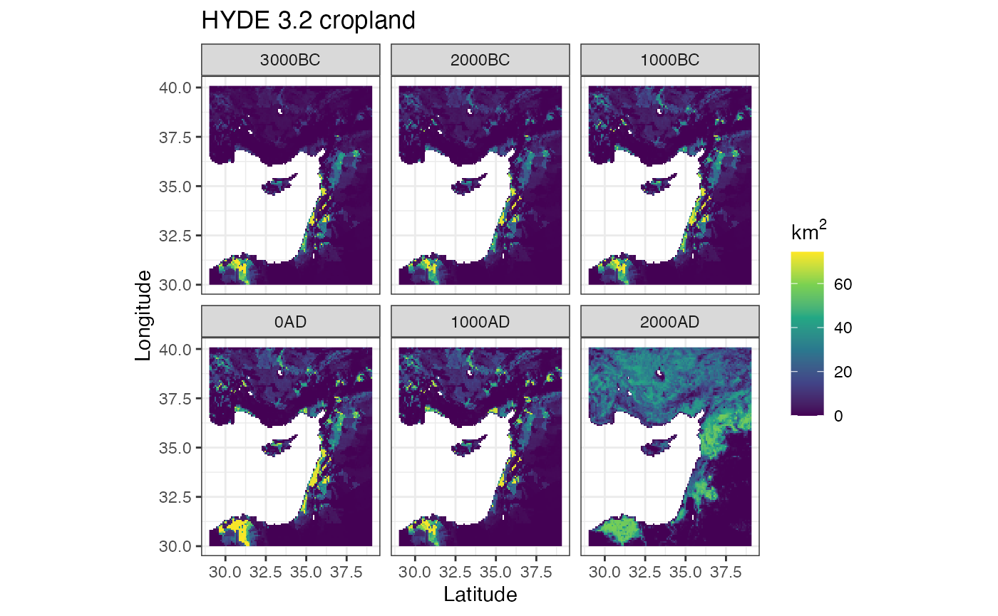
You can easily animate these data using gganimate.
ggplot() +
  geom_stars(data = filter(hyde_med)) +
  coord_quickmap() +
  scale_fill_viridis_c(na.value = NA, name = expression(km^2)) +
  theme_bw() +
  # use transition_states() from gganimate instead of facet_wrap
  gganimate::transition_states(time) +
  labs(title = 'HYDE 3.2 land use', subtitle = 'Cropland at {closest_state}', x = 'Latitude', y = 'Longitude')
By default, geom_stars will only plot the first attribute. If you’d like to plot multiple attributes at a time, the easiest way is to convert the attributes to an extra dimension.
ggplot() +
  geom_stars(data = merge(hyde_med[c(1:2,5),,,])) +
  facet_grid(attributes~time) +
  coord_quickmap() +
  scale_fill_viridis_c(na.value = NA, name = expression(km^2)) +
  theme_bw() +
  labs(title = 'HYDE 3.2 land use', x = 'Latitude', y = 'Longitude')
#> Warning: Removed 81396 rows containing missing values (geom_raster).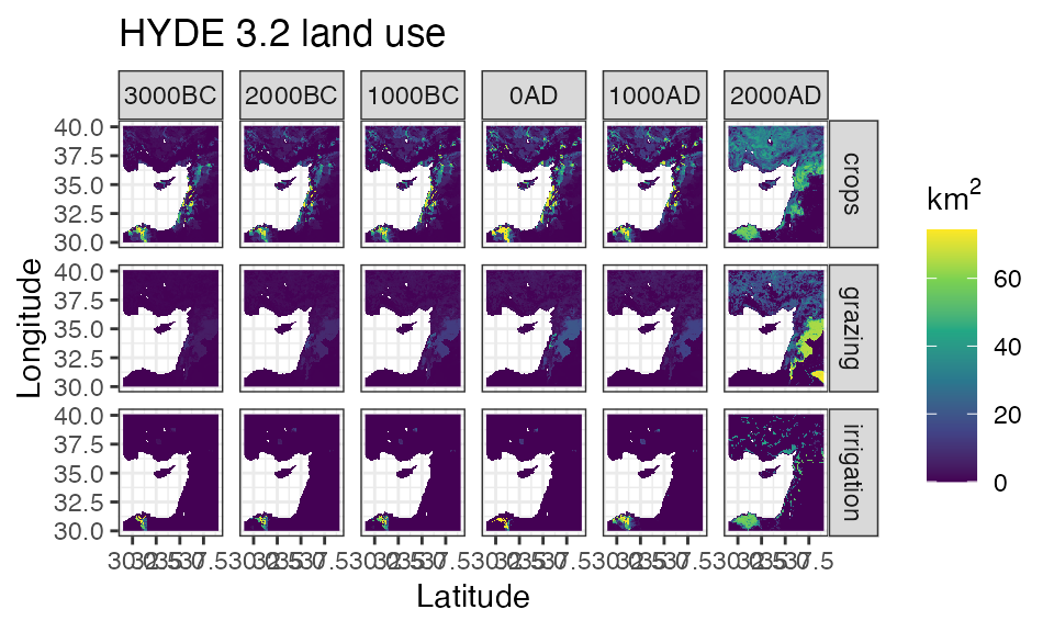
Anthromes classification
anthromes <- anthrome_classify(hyde_med, inputs_med)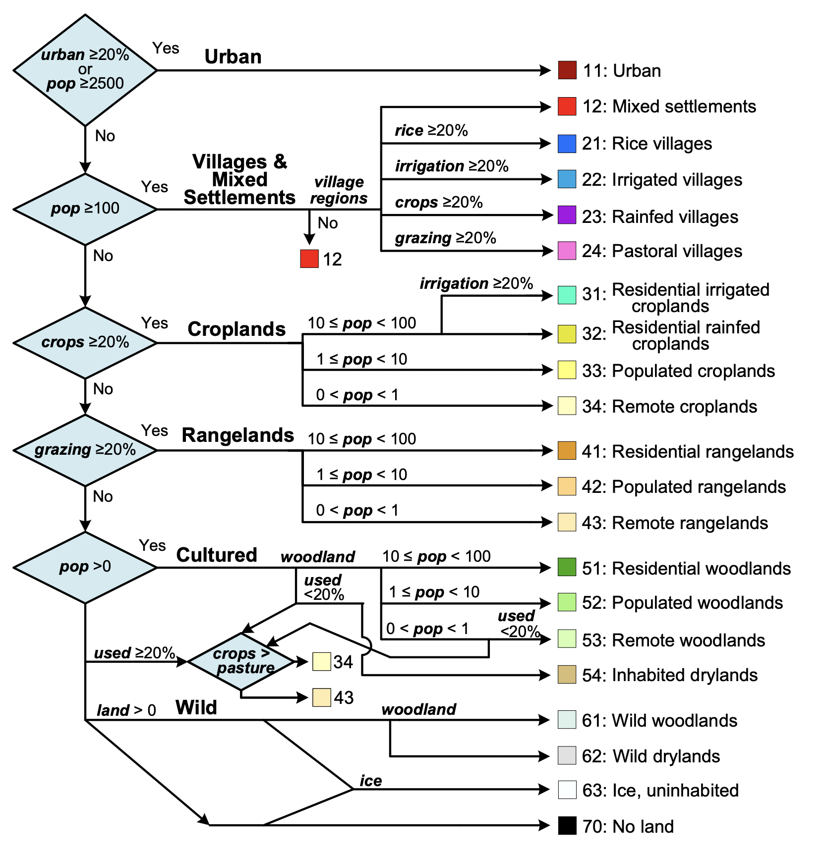
ggplot() +
  geom_stars(data = anthromes) +
  facet_wrap(~time) +
  coord_quickmap() +
  scale_fill_manual(values = anthrome_colors(), drop = TRUE) +
  theme_bw() +
  labs(title = 'Anthromes-12k', x = 'Latitude', y = 'Longitude')
#> Warning: Removed 27132 rows containing missing values (geom_raster).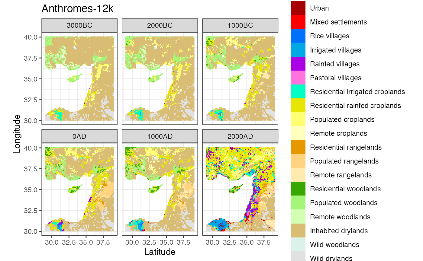
Discrete Global Grids
Rasters are great, but a hexagonal discrete global grid system would keep the cell areas the same and better represent shapes over the Earth’s surface.
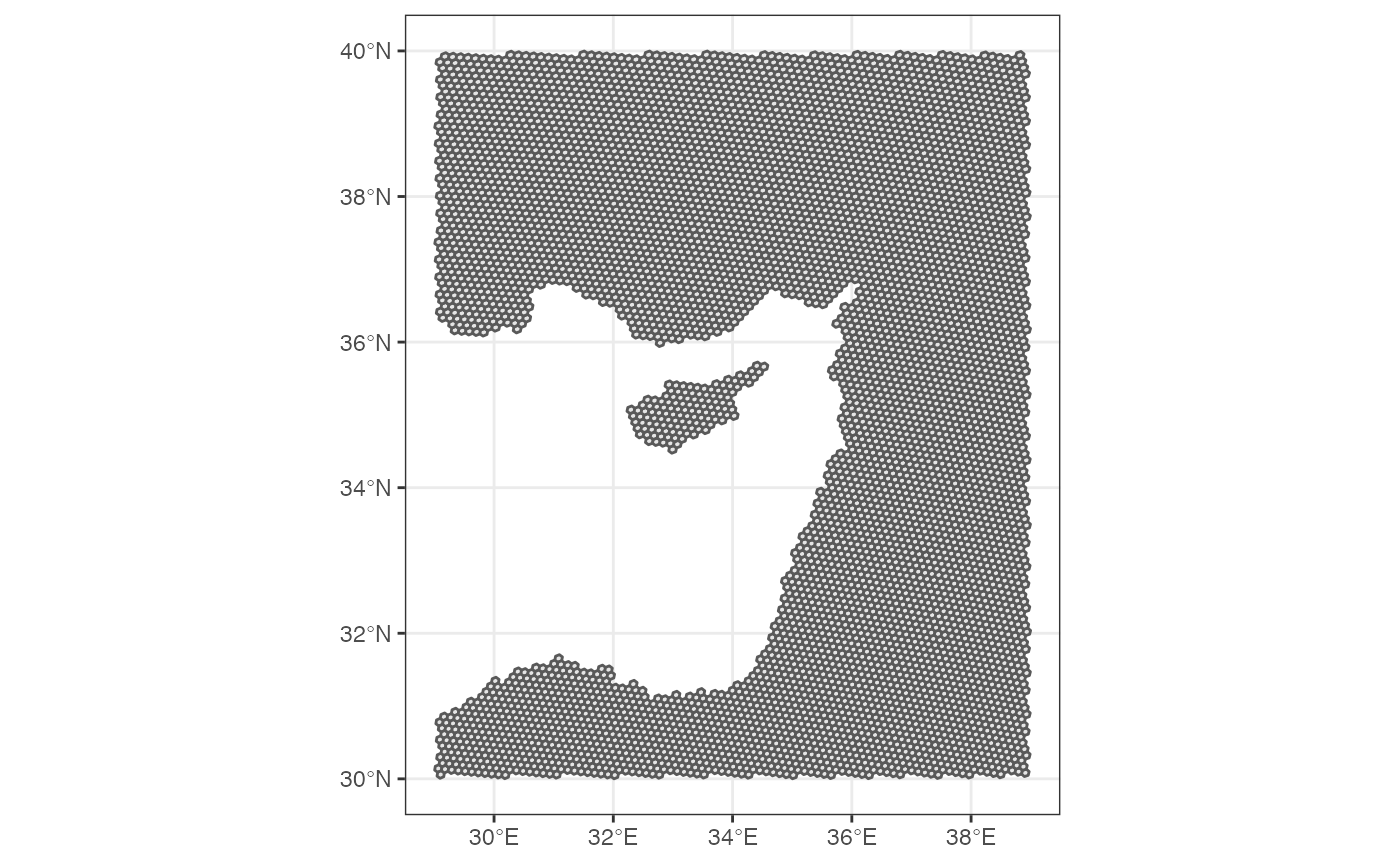
Use the dgg_extract() function to extract the HYDE 3.2 data using the DGG hexagons. It uses exactextractr under the hood, which prints a progress bar by default.
crops <- dgg_extract(hyde_med, dgg_med, 'crops', fun = 'sum')
ggplot() +
  geom_stars(data = crops) +
  facet_wrap(~time) +
  scale_fill_viridis_c(na.value = NA, name = expression(km^2)) +
  theme_bw() +
  labs(title = 'HYDE 3.2 cropland', subtitle = 'Discrete global grid system', x = 'Latitude', y = 'Longitude')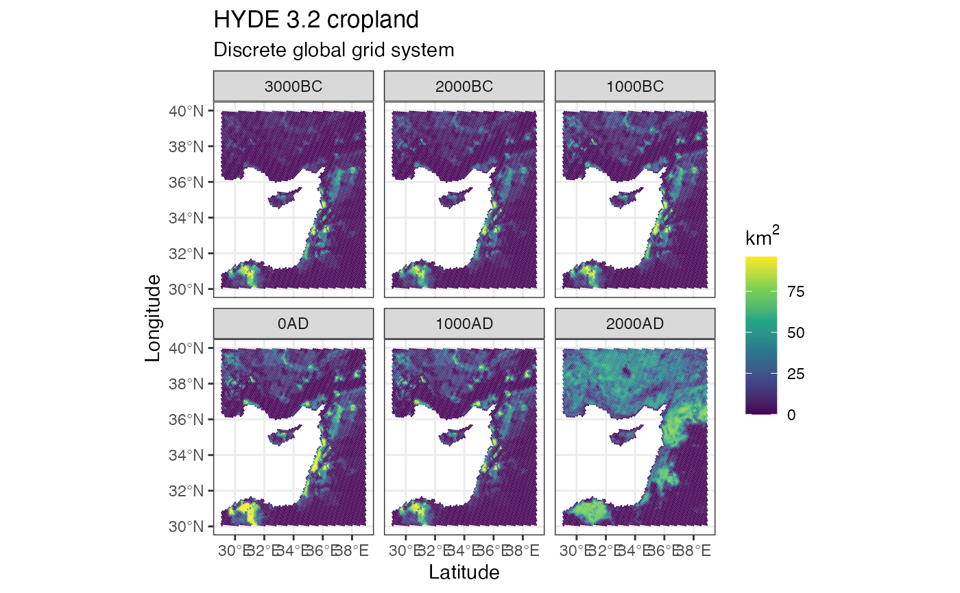
Let’s compare it to the 5’ raster
a <- ggplot() +
  geom_stars(data = hyde_med[,,,5]) +
  coord_quickmap() +
  scale_fill_viridis_c(na.value = NA, name = expression(km^2)) +
  theme_bw() +
  labs(title = 'HYDE 3.2 cropland', x = 'Latitude', y = 'Longitude')

b <- ggplot() +
  geom_stars(data = crops[,,5]) +
  scale_fill_viridis_c(na.value = NA, name = expression(km^2)) +
  theme_bw() +
  labs(title = '', subtitle = 'Discrete global grid system', x = 'Latitude', y = 'Longitude')

a + b
#> Warning: Removed 4522 rows containing missing values (geom_raster).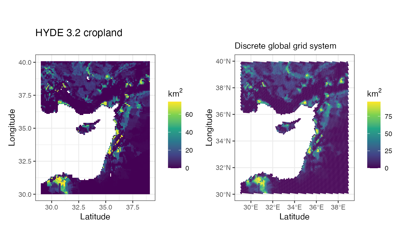
Map this function over the list of HYDE variable names.
hyde_dgg <- names(hyde_med) %>%
  purrr::map(~dgg_extract(hyde_med, dgg_med, var = ., fun = 'sum')) %>%
  do.call(c, .)
ggplot() +
  geom_stars(data = merge(hyde_dgg[c(1:2,5),,])) +
  facet_grid(attributes~time) +
  scale_fill_viridis_c(na.value = NA, name = expression(km^2)) +
  theme_bw() +
  labs(title = 'HYDE 3.2 land use', x = 'Latitude', y = 'Longitude')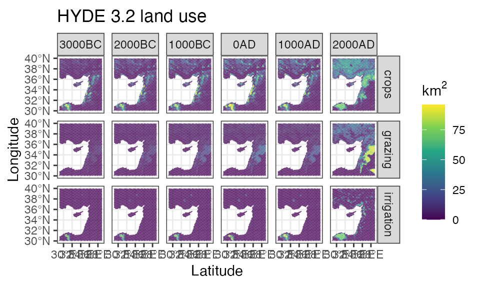
And extract the fixed inputs as well.
# fold this into dgg_extract too?
inputs_dgg <- dgg_extract(merge(inputs_med), dgg_med, fun = c('sum', 'mode')) %>%
   dplyr::select(land_area = sum.land_area,
                pot_veg =  mode.pot_veg,
                pot_vill = mode.pot_vill,
                regions = mode.regions,
                iso = mode.iso)
Apply the anthromes classifier to each level
anthromes_dgg <- anthrome_classify(hyde_dgg, inputs_dgg)
ggplot() +
  geom_stars(data = anthromes_dgg) +
  facet_wrap(~time) +
  scale_fill_manual(values = anthrome_colors(), drop = TRUE) +
  theme_bw() +
  labs(title = 'Anthromes-12k DGG', x = 'Latitude', y = 'Longitude')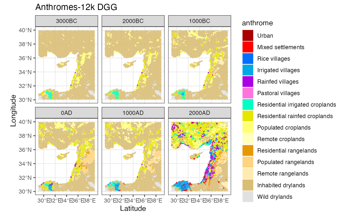
 ggplot() +
  geom_stars(data = anthromes[,,,6]) +
  coord_quickmap() +
  scale_fill_manual(values = anthrome_colors(), drop = TRUE) +
  theme_bw() +
  labs(title = 'Anthromes-12k', x = 'Latitude', y = 'Longitude')
#> Warning: Removed 4522 rows containing missing values (geom_raster).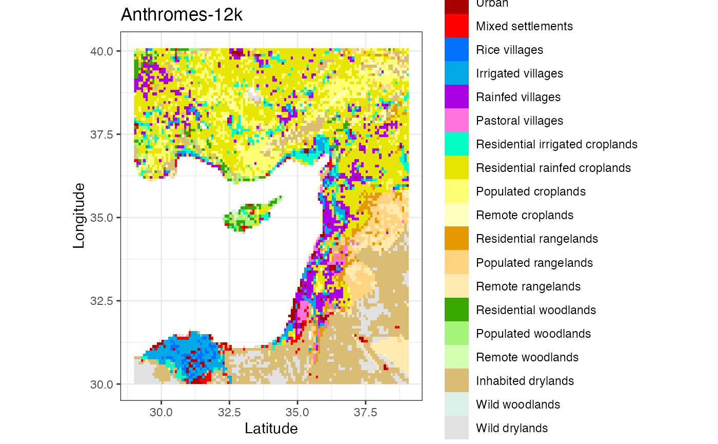
ggplot() +
  geom_stars(data = anthromes_dgg[,,6]) +
  scale_fill_manual(values = anthrome_colors(), drop = TRUE) +
  theme_bw() +
  labs(title = 'Anthromes-12k DGG', x = 'Latitude', y = 'Longitude')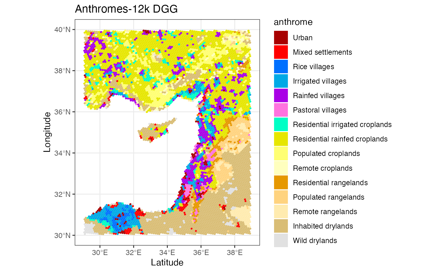
Summary statistics
Use the anthrome_summary() function to produce formatted summary tables of the percent land area of under each anthrome type for each time period.
anthrome_summary(anthromes_dgg, inputs_dgg)
#> # A tibble: 15 x 7
#>    anthrome             `3000BC`  `2000BC`  `1000BC`     `0AD` `1000AD` `2000AD`
#>    <fct>                     [%]       [%]       [%]       [%]      [%]      [%]
#>  1 Urban               0.000000…  0.00000…  0.00000…  0.00000…  0.0000…  1.2092…
#>  2 Mixed settlements   0.000000…  0.00000…  0.01468…  0.02904…  0.1275…  1.8119…
#>  3 Rice villages       0.000000…  0.00000…  0.01468…  0.11746…  0.1908…  1.3286…
#>  4 Irrigated villages  0.000000…  0.01468…  0.26714…  0.64607…  1.1190…  5.8866…
#>  5 Rainfed villages    0.079573…  0.09408…  0.09408…  0.55637…  0.1234…  8.1408…
#>  6 Pastoral villages   0.000000…  0.00000…  0.00000…  0.00000…  0.0000…  1.1366…
#>  7 Residential irrig…  1.380180…  1.59076…  1.45577…  0.66076…  1.2801…  4.0472…
#>  8 Residential rainf…  2.382202…  3.57978…  7.99906… 13.38962… 10.3766… 31.2408…
#>  9 Populated croplan…  5.224924…  5.80186…  5.35229…  4.31160…  5.0813…  7.8481…
#> 10 Remote croplands    0.942821…  1.83371…  3.29280…  4.19957…  5.1464…  2.0355…
#> 11 Residential range…  0.000000…  0.01468…  0.08810…  1.42428…  0.2053…  2.6472…
#> 12 Populated rangela…  0.000000…  0.04352…  0.10226…  5.55511…  3.3620…  4.2654…
#> 13 Remote rangelands   0.175879…  0.27896…  2.18518…  1.09183…  2.5056…  3.1843…
#> 14 Inhabited drylands 87.099973… 84.03346… 76.42858… 65.53546… 68.0719… 23.7548…
#> 15 Wild drylands       2.714443…  2.71444…  2.70534…  2.48276…  2.4093…  1.4622…
anthrome_summary() also has a “by” argument, which adds an additional grouping factor. The resulting summaries are now in percent of land area under each anthrome in each time period in each of the grouping variables.
anthrome_summary(anthromes_dgg,
                 mutate(inputs_dgg, pot_veg = as.factor(pot_veg)),
                 by = pot_veg)
#> # A tibble: 108 x 8
#>    pot_veg anthrome       `3000BC` `2000BC` `1000BC`     `0AD` `1000AD` `2000AD`
#>    <fct>   <fct>               [%]      [%]      [%]       [%]      [%]      [%]
#>  1 3       Urban          0.000000 0.000000 0.000000  0.000000  0.0000…  0.5744…
#>  2 3       Mixed settlem… 0.000000 0.000000 0.000000  0.000000  0.0000…  1.9553…
#>  3 3       Irrigated vil… 0.000000 0.000000 0.000000  0.000000  0.0000…  4.8957…
#>  4 3       Rainfed villa… 0.000000 0.000000 0.000000  0.000000  0.0000… 11.3291…
#>  5 3       Pastoral vill… 0.000000 0.000000 0.000000  0.000000  0.0000…  0.0381…
#>  6 3       Residential i… 0.000000 0.000000 0.000000  0.000000  0.0000…  5.6263…
#>  7 3       Residential r… 0.128218 1.835374 9.421701 16.714982 17.7109… 41.5960…
#>  8 3       Populated cro… 5.265605 9.852276 6.535757  3.962339  3.5436… 10.9493…
#>  9 3       Remote cropla… 0.520486 1.349584 3.454024  2.503946  4.4823…  4.1192…
#> 10 3       Residential r… 0.000000 0.000000 0.000000  0.000000  0.0000…  0.1499…
#> # … with 98 more rows
anthrome_summary(anthromes_dgg,
                 mutate(inputs_dgg, iso = as.factor(iso)),
                 by = iso)
#> # A tibble: 97 x 8
#>    iso   anthrome        `3000BC`  `2000BC`  `1000BC`    `0AD` `1000AD` `2000AD`
#>    <fct> <fct>                [%]       [%]       [%]      [%]      [%]      [%]
#>  1 196   Urban            0.0000…   0.0000…   0.0000…   0.000…   0.000…   0.802…
#>  2 196   Mixed settlem…   0.0000…   0.0000…   0.0000…   0.000…   0.000…   7.613…
#>  3 196   Rainfed villa…   0.0000…   0.0000…   0.0000…   0.000…   0.000…   3.166…
#>  4 196   Residential i…   0.0000…   0.0000…   0.0000…   0.000…   0.000…   3.837…
#>  5 196   Residential r…   0.8610…   1.2449…   6.6818…  19.042…  11.691…  22.508…
#>  6 196   Populated cro…  19.8878…  19.5039…  18.9807…  14.176…  13.169…   0.000…
#>  7 196   Remote cropla…   0.0000…   0.0000…   5.0703…   0.000…   5.162…   0.000…
#>  8 196   Inhabited dry…  78.8944…  78.8944…  68.9105…  66.424…  69.620…  61.715…
#>  9 196   Wild drylands    0.3565…   0.3565…   0.3565…   0.356…   0.356…   0.356…
#> 10 368   Inhabited dry… 100.0000… 100.0000… 100.0000… 100.000… 100.000… 100.000…
#> # … with 87 more rows
You can also use the hyde_summary() function to extract population estimates from HYDE.
hyde_summary(hyde_dgg, inputs_dgg) %>%
  ggplot(aes(time, pop, group = 1)) +
  geom_point() +
  stat_summary(fun.y=sum, geom="line") +
  theme_bw()
#> Warning: `fun.y` is deprecated. Use `fun` instead.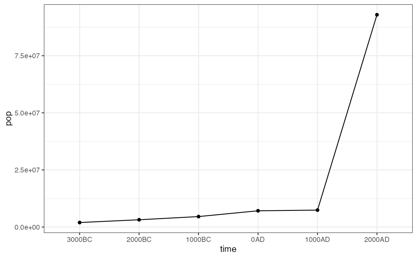
Statistical modeling
As stars objects, the data can be easily coerced to a tibble for statistical analysis.
pc <- hyde_dgg %>%
  as_tibble() %>%
  select(-geometry, -time) %>%
  prcomp(scale. = TRUE)

pc
#> Standard deviations (1, .., p=6):
#> [1] 1.4868954 1.1714271 1.0232623 0.8859689 0.6578860 0.3899745
#>
#> Rotation (n x k) = (6 x 6):
#>                   PC1         PC2         PC3          PC4          PC5
#> crops      0.36236910  0.47843009  0.24372900  0.483283668 -0.588754240
#> grazing    0.06660792  0.06155533  0.90093980 -0.402903801  0.133138492
#> rice       0.34601137  0.30038089 -0.33936869 -0.756940229 -0.302341903
#> pop        0.55928161 -0.40862354 -0.01419267  0.004915589 -0.006758806
#> irrigation 0.43822311  0.47512354 -0.10597994  0.150900594  0.737391518
#> urban      0.48958425 -0.53326479  0.04795170  0.091387977 -0.020976839
#>                     PC6
#> crops      -0.013957237
#> grazing     0.004947393
#> rice       -0.102504680
#> pop         0.721082246
#> irrigation -0.066851576
#> urban      -0.681795256
knitr::knit_exit()