Projected warming will exceed the long-term thermal limits of rice cultivation
Authors
Affiliations
Nicolas Gauthier
University of Florida, Florida Museum of Natural History
Ornob Alam
New York University, Center for Genomics and Systems Biology
Michael D. Purugganan
New York University, Center for Genomics and Systems Biology
New York University, Center for the Study of the Ancient World
Jade d’Alpoim-Guedes
University of Washington, Department of Anthropology
Abstract
Rice is a staple food for a significant portion of the global population, particularly in Asia, where over one billion people rely on it for daily subsistence. Understanding rice’s historical thermal limits is imperative for predicting how it will respond to future shifts in global climate. Here, we integrate diverse records of contemporary rice cultivation extent, archaeological data spanning rice’s long-term history since its earliest cultivation, and temperature projections for the past, present, and future to assess how warm temperatures have influenced and may continue to influence rice’s geographical distribution, productivity, and the adaptive strategies employed by human societies to sustain this important crop. Our findings indicate a consistent pattern over the past 10,000 years: domesticated Asian rice varieties have seldom thrived in regions where the mean annual temperature exceeds 28°C or warm-season maximum temperature exceeds 33°C. By the end of this century, climate projections estimate that the land area exceeding this thermal threshold in Asia’s major rice-producing nations could expand by ten to thirty times. Our findings have significant implications for global food security, as regions heavily reliant on rice cultivation may encounter unprecedented challenges in staple crop production under projected warming.
── Attaching core tidyverse packages ──────────────────────── tidyverse 2.0.0 ──
✔ dplyr     1.1.4     ✔ readr     2.1.5
✔ forcats   1.0.0     ✔ stringr   1.5.1
✔ ggplot2   3.5.2     ✔ tibble    3.3.0
✔ lubridate 1.9.4     ✔ tidyr     1.3.1
✔ purrr     1.1.0
── Conflicts ────────────────────────────────────────── tidyverse_conflicts() ──
✖ dplyr::filter() masks stats::filter()
✖ dplyr::lag()    masks stats::lag()
ℹ Use the conflicted package (<http://conflicted.r-lib.org/>) to force all conflicts to become errors
library(sf)
Linking to GEOS 3.14.0, GDAL 3.11.3, PROJ 9.6.0; sf_use_s2() is TRUE
WARNING: different compile-time and runtime versions for GEOS found:
Linked against: 3.14.0-CAPI-1.20.4 compiled against: 3.13.1-CAPI-1.19.2
It is probably a good idea to reinstall sf (and maybe lwgeom too)
library(stars)
Loading required package: abind
library(ggridges)library(patchwork)# if installing the rnaturalearth libraries yields an error, uncomment and run the lines below# remotes::install_github("ropensci/rnaturalearthhires") library(rnaturalearth)library(rnaturalearthdata)
Attaching package: 'rnaturalearthdata'

The following object is masked from 'package:rnaturalearth':

    countries110
library(here)
here() starts at /Users/nick/UFL Dropbox/Nick Gauthier/Projects/rice
library(units)
udunits database from /Users/nick/Library/Caches/org.R-project.R/R/renv/cache/v5/macos/R-4.4/aarch64-apple-darwin20/units/0.8-7/5d0b024902d5da97a2b64f002e92a869/units/share/udunits/udunits2.xml
library(eks)library(gt)theme_set(theme_bw())# define the study areaasia_bbox_sf <-st_bbox(c(xmin =60, xmax =150, ymin =-11, ymax =54), crs =4326)world_bbox_sf <-st_bbox(c(xmin =-130, xmax =155, ymin =-40, ymax =60), crs =4326)# get country boundaries shapefile for plottingsf_use_s2(FALSE)
Spherical geometry (s2) switched off
countries <-ne_countries(scale ='large') %>%st_crop(asia_bbox_sf)
although coordinates are longitude/latitude, st_intersection assumes that they
are planar
Warning: attribute variables are assumed to be spatially constant throughout
all geometries
Members of the grass family (Poaceae), which include staples like rice, maize, wheat, and barley, provide a majority of the global human caloric intake. However, these crops face a looming threat: the rate of anticipated climate change eclipses that of historical niche adaptations in grasses. By 2070, temperatures are projected to rise at a rate 5,000 times faster than what most varieties of Poaceae have experienced throughout their evolution (1). Historically, Poaceae experienced temperature shifts ranging from 1-8°C per million years, yet future projections anticipate changes as swift as 0.02°C annually (1). Among these vital crops, domesticated Asian rice (Oryza sativa) serves as a primary food source for over half the global population. More than 90% of the world’s rice is grown in Asia, and one fifth of the world’s population—more than 1 billion people—depend on rice cultivation for their livelihood.
Oryza sativa has a deep history of cultivation and domestication beginning at least 7,000 years ago. Over the course of its domestication and subsequent spread, Asian rice has made several adaptations to changes in climate and has expanded well beyond its original range of cultivation. Yet despite this expansion, rice exhibits a high degree of niche conservatism compared to its wild progenitor (2). Although human selection—and, in recent decades, scientific breeding—can accelerate the development of new traits far more rapidly than the thousands of years wild plant species often require to adapt to new climatic conditions, these advances have not successfully expanded rice’s thermal tolerance. Notably, as global temperatures rise, rice farming has shifted from warmer areas to cooler ones rather than adapting to increased heat (3). Apparent increases in rice’s harvested area over recent decades largely reflect advances in farming technology rather than an expansion of its climatic tolerance. For example, rice cultivation in the People’s Republic of China has gradually extended northward from Central China into cooler regions, a shift that, combined with intensified irrigation in the country’s hottest zones, has modestly increased rice yields and masked the adverse effects of rising temperatures (3, 4).
While some areas may benefit from warming temperatures (5), this trend is not universal. In many regions, smallholder farmers rely on rice cultivation as their main source of income. Indeed, mismatches between rice-harvested areas and overall environmental suitability suggest that subsistence farming in low-income regions has already stretched rice cultivation to its climatic boundaries (6). To put this into perspective, projections indicate that 15-40% of India’s current rainfed rice cultivation zones will experience a reduction in climatic suitability by 2050 (7). Since 1974, 88% of rice-harvested areas show significant shifts in yield due to climatic factors, with climate change reducing consumable food calories from rice by 0.4% compared to historical climate conditions (8).
However, these findings are constrained by the current distributions of rice cultivation and prevailing temperature. Few regions of the world today experience the elevated temperatures projected in many future climate-change scenarios. This makes it challenging to distinguish between inherent thermal limits for rice growth and the practical geographic constraints set by recent temperature distributions (9, 10). Global temperatures have already exceeded known temperatures over the past 2,000 years and we are living in the warmest centuries of at least the past 100,000 years (11). Contemporary studies of the thermal niche of rice have provided crucial insights into specific regions and production systems, but those with a global scope have often been reliant on limited datasets that may not capture the full diversity of rice distributions. Challenges include the potential underrepresentation of temperate rice varieties in China, uneven sampling of rainfed or upland varieties, and the geographic scope of the studies, which do not always encompass broad thermal ranges (4, 7, 9). Archaeological studies have been instrumental in documenting the timing and geographic trajectory of rice’s domestication and spread across Asia (12–16). Recent integration of archaeological rice records with spatial paleoclimate reconstructions has revealed that climate change played a major role in the early diversification and spread of rice (17, 18), but the implications for rice’s future adaptability have yet to be fully explored.
Here, we integrate multiple lines of evidence from the extensive history of rice cultivation to characterize the thermal range of rice and gauge its potential adaptability to impending climate changes. By integrating diverse records of the current extent of rice cultivation with archaeological data on the distribution of rice since its earliest cultivation and domestication, we aim to establish O. sativa’s thermal limits—the temperature conditions under which rice has been consistently cultivated throughout its domestication history. We estimate long-term thermal limits associated with rice cultivation by comparing contemporary estimates of rice extent with well-dated archaeological rice occurrences, and complement this with genetic analyses of adaptation potential in rice subspecies. We focus specifically on Asian rice (O. sativa) rather than African rice (O. glaberrima), as Asian rice comprises the vast majority of global production and consumption and has the extensive archaeological record necessary for long-term analysis. We use these results to assess the impact of projected climate changes by the end of this century. Together, our analyses confirm that imminent changes in climate conditions may force large regions of today’s primary rice producers to confront mean annual, seasonal, and monthly peak temperatures unprecedented in the history of rice cultivation and domestication.
Results
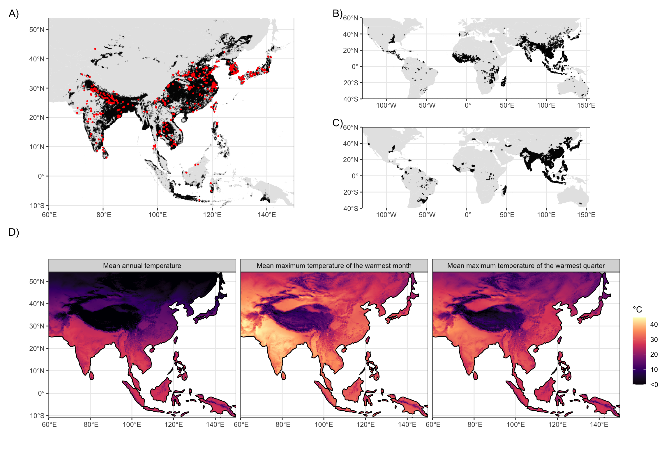
We assess thermal limits on rice growth by comparing contemporary rice extents estimated from satellite imagery, agricultural censuses, and herbarium collections to indicators of annual and seasonal temperature (Figure 1). Our analysis combines present-day rice extent data from diverse sources: satellite-based assessments of paddy rice extent in Asia (19), hybrid satellite/census evaluations of global paddy rice cropping areas around the year 2000 (20), and global point occurrences derived from herbarium records and germplasm accessions (22). These datasets span a range of spatial scales, time periods, production systems (e.g. irrigated vs. rainfed), and data collection methods with complementary biases, allowing us to test the robustness of these thermal limits across methodologically independent data sources. We supplement this empirical work with reviews of rice’s response to warm temperatures from prior field and lab-based agronomic studies.
Warning: Removed 309243 rows containing missing values or values outside the scale range
(`geom_raster()`).
Figure 1: Observed rice extent data and thermal predictors. A) Map of lowland rice extent in Asia from the International Rice Research Institute based on estimates from MODIS satellite imagery (19) (black) overlain by archaeological sites with evidence for rice cultivation (red). B) Point based rice occurrences from global herbarium records and genetic accessions. C) Satellite-based estimates of rice cropped area in the year 2000 from (20). D) Maps of mean annual temperature, mean maximum daily temperature of the warmest month, and mean maximum daily temperature of the warmest quarter from CHELSA V2.1 averages for 1981-2010 (23–25).
We define the “thermal limits” of rice cultivation as the 95% central range of three temperature indicators at all sampled rice occurrence locations in a given dataset—the temperature thresholds beyond which the likelihood of rice cultivation significantly deceases due to a combination of physiological, cultural, and economic factors. This empirical approach emphasizes the long-term feasibility of crop cultivation rather than short-term variations in yield or harvested area. By focusing on these broader climatic measures, we can integrate a wider array of data sources from the past and present to reveal the upper temperature thresholds of rice cultivation over time.
Our approach offers a parsimonious tool for estimating future crop suitability (26, 27) that complements process-based crop models. While such models can extrapolate yield responses to climate change, they are sensitive to assumptions about meteorological inputs, agronomic and physiological parameters, and cultural practices like planting dates and varietal preferences over the long term (28–32). Translating these localized projections to global scales introduces additional challenges, as does calibrating and validating their outputs using limited and inconsistent yield data from the recent or more distant past. Ultimately, a better understanding of baseline thermal limits and their uncertainty through time and space can contribute to the development of future process-based models, many of which incorporate temperature thresholds for pivotal crop development phases.
We focus primarily on temperature rather than precipitation or soil moisture, as water availability can be more readily controlled through human interventions such as irrigation and paddy field construction. These adaptations have allowed rice cultivation to expand beyond its original aquatic and semi-aquatic environments. In contrast, adapting to new thermal conditions is more challenging and often requires changes in planting dates or crop varieties, which have their own limitations, particularly in higher latitudes where daylight variations restrict growing seasons.
Contemporary rice extents are constrained by high temperatures
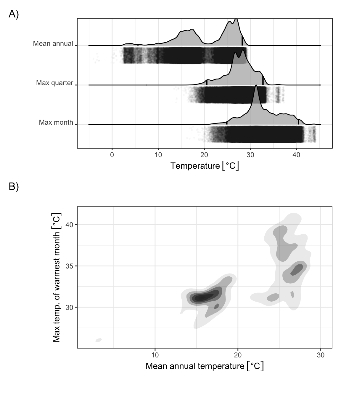
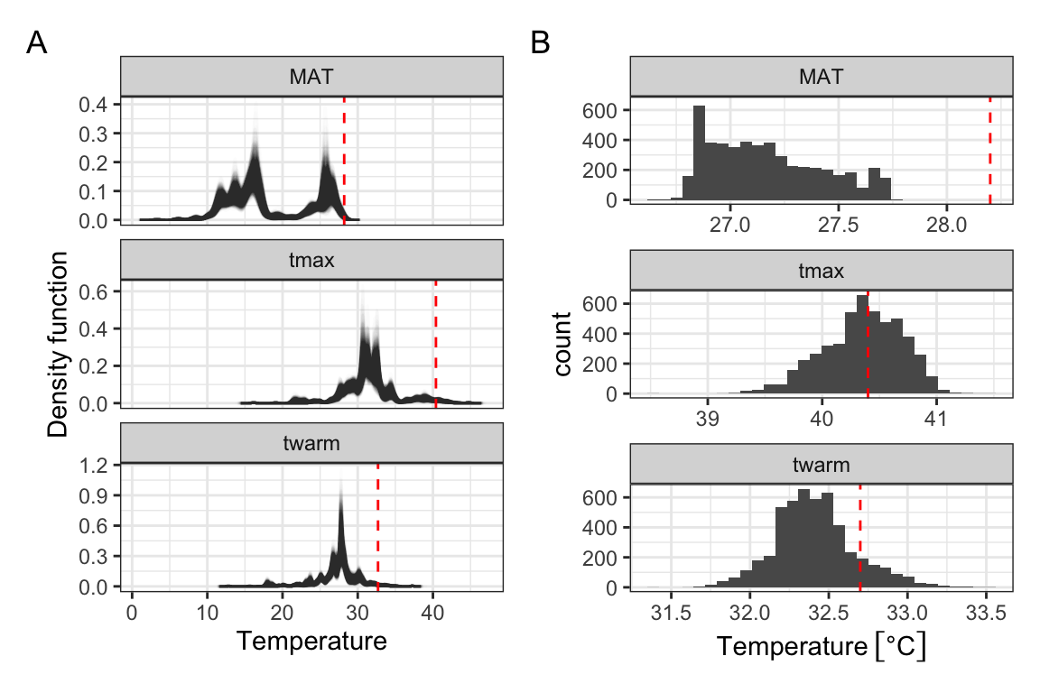
Contemporary rice extents fall within a relatively restricted thermal range. We use mean annual temperature (MAT), mean maximum daily temperature of the warmest quarter (TWARM), and mean maximum daily temperature of the warmest month (TMAX) to estimate upper boundary temperatures for contemporary rice occurrences. The vast majority of contemporary rice is grown in regions with MAT below 28.2℃, TWARM of 32.7℃, and TMAX of 40.4℃ (Figure 2). Although we primarily report results from the satellite-based estimates of lowland rice extent over Asia produced by the International Rice Research Institute (19) due to its favorable balance of spatial resolution and extent, results from other rice extent datasets with variable spatial extent, resolution, and time span are consistent with these findings (Supplementary Table 1). There is much more variability across data sources in lower temperature thresholds—reflecting the greater adaptability of rice to colder temperatures through breeding, management, and growing season—than upper temperature thresholds.
Warning: Use of the `vline_size` or `size` aesthetic are deprecated, please use
`linewidth` instead of `size` and `vline_width` instead of `vline_size`.
Warning: Use of the `vline_size` aesthetics is deprecated, please use
`vline_width` instead of `vline_size`.
Warning: Use of the `vline_size` aesthetics is deprecated, please use
`vline_width` instead of `vline_size`.
Warning: Use of the `vline_size` aesthetics is deprecated, please use
`vline_width` instead of `vline_size`.
Warning: Removed 41 rows containing non-finite outside the scale range
(`stat_density2d()`).
Figure 2: Kernel density estimates of temperature distributions over rice growing landscapes in Asia. A) One-dimensional kernel density estimates of mean annual temperature and mean maximum daily temperature of the warmest month in grid cells with lowland rice crops, based on data from the International Rice Research Institute (fig. 1). Vertical black lines indicate the 95% central range of the temperature values, and transparent black points indicate the raw occurrence data used in the calculation of the kernel density estimates. B) Two dimensional kernel density estimates for the same variables as in A.
These empirical thresholds are consistent with physiological parameters inferred from field-scale agronomic studies and expert knowledge, which estimate that the optimum temperature range for reproductive yield in rice is 23℃-26℃, biomass and pollen viability declines when maximum temperatures exceed 33℃, and crop viability reaches zero at approximately 40℃ when photosynthesis begins to shut down in C3 plants like rice (33). In other words, rice today is rarely grown in regions where the mean annual temperature exceeds its optimum temperature for reproduction, warm-season maximum temperatures exceed its optimum for pollen viability, and summer heat extremes will reliably stop photosynthesis.
These broad climate indices, while not capturing all nuances of local growing conditions, serve as useful heuristics for identifying regions prone to thermal stress. This approach provides a complementary perspective to typical empirical crop models, which often use fixed monthly or seasonal predictors tied to the timing of the growing season. These predictors depend on planting dates, which are themselves cultural adaptations to past and present climate. As planting times and growing seasons shift with climate change, statistical analyses based solely on “growing season” temperatures may become less reliable for long-term historical comparison. Our approach provides a stable benchmark for integrating archaeological and contemporary data across different time periods and cultivation practices, helping identify where adaptations in growing seasons, crop types, genetics, or irrigation practices may become necessary.
High-temperature constraints are consistent across 9,000 years of rice cultivation
Although upper temperature limits on rice growth estimated from contemporary crop occurrences are consistent with previous agronomic studies, it is not yet clear how well these thresholds will predict crop responses to future temperature changes. For example, there are few places today that experience mean annual temperatures beyond 28℃ (Supplementary Figure 7), and contemporary correlations between mean annual temperatures and monthly or seasonal extremes may not hold in a changing climate. The archaeological record of rice cultivation in Asia, including direct dates of botanical remains and contextual dating of concurrent archaeological sites, provides a unique opportunity to assess the robustness of these temperature limits over the long term. During the mid Holocene ca 8000-4000 calibrated years BP (cal. BP), warm-season temperatures were generally warmer than present, reflecting increased summertime insolation in the Northern Hemisphere due to shifts in Earth’s orbit and consequent feedbacks in the global climate system (34). Although not an exact analogue for projected future warming caused by greenhouse gas emissions, this period provides a baseline for rice’s response to shifting climates during the critical period of its domestication and dispersal.
O. sativa has been domesticated a number of times in prehistory. Archaeological data shows that wild forms of rice were distributed as far north as northern China in the early Holocene (ca 9000 cal. BP) and gathered by foraging populations (35). Tropical varieties of O. sativa japonica were first cultivated in the middle and lower Yangtze and Yellow River valleys in China by at least 7000 cal. BP (36–38) (Figure 3 A), where they began to exhibit traits of domestication (e.g. the development of a non-shattering rachis) by roughly 5000 cal. BP (12, 39). Oryza sativa indica rices on the other hand were likely domesticated in South Asia sometime around 4000 cal. BP (40, 41), after which it spread throughout southeast Asia and China (Figure 3 A). There is substantially less archaeobotanical data, however, that speaks to the cultivation and subsequent domestication of this subspecies (41). This period of initial cultivation and domestication corresponds to the warmer mid-Holocene thermal maximum.
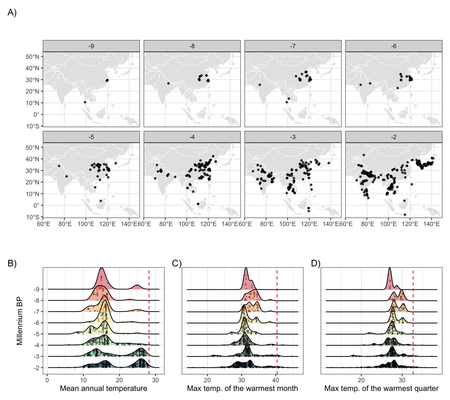
Between roughly 5000-4000 BP, rice spread both north- and eastward in China (42, 43) and westward onto the Chengdu Plain (44) and highlands of Southwest China (45, 46) (Figure 3 A). Genetic and paleoclimate modeling have suggested that regional cooling around 4200 BP played an important role in this spread resulting in strong pressure for tropical O. japonica to develop temperate adaptations (18). Estimated divergence time for tropical and temperate O. japonica is indeed estimated at around 4100 BP (18). Following the development of temperate O. japonica varieties, rice spread to both Korea (47, 48) and Japan (14) (Figure 3 A). At the same time, it appears that the area that tropical varieties of O. japonica were able to occupy shifted southwards to southern China (49, 50) and southeast Asia (51–53) (Figure 3 A), largely representing the dispersal of existing tropical varieties rather than novel adaptations to new thermal extremes. Indeed between 4000-3000 BP, rice farming spread into Thailand (53), Laos, Bhutan, and then via maritime routes to Taiwan, the Philippines, Malaysia, and Indonesia (18) (Figure 3 A). A clear split in the distribution of rice with regards to temperature is evident following 4000 BP and we see a clear split into two populations: temperate varieties which occupy a mean annual temperature niche between roughly 8-18℃ and tropical varieties which occupy a niche between 22-27℃ (Figure 3 B).
Figure 3: Archaeological remains of rice and corresponding temperature distributions throughout the Holocene. A.) Archaeological records of rice distribution over time. See Materials and Methods for archaeological data sources. Time units are thousands of years before present (1950 CE). B.) Kernel density estimates of the thermal distribution by millennium, with raw data points indicated in black and contemporary rice thermal limits in red. Rice occurrence data were derived from sources listed in the Materials and Methods. Temperature data are derived from CHELSA-TraCE21k V1.0 (Karger et al. 2023).
These repeated instances of rice’s diversification and shifting ranges throughout its history primarily reflect genetic and cultural adaptations to cooler temperatures and shorter growing seasons. In contrast, movements into warmer regions generally involved range shifts by varieties already suited to such conditions rather than novel adaptations. Across these shifts, rice’s upper temperature limits have remained consistent. Out of 803 archaeological sites with rice remains, none have experienced MAT of greater than 28.2℃ during the Holocene (Figure 3 B), in spite of warmer summer temperatures overall. Only a handful of sites experienced a TMAX of greater than 40.4℃ (Figure 3 C), primarily in arid regions of northern India and Pakistan where archaeological dating is less certain and long-distance trade rather than local cultivation is more plausible. Regardless, the archaeological record of rice cultivation is consistent with the thermal limits estimated from contemporary data, and these results are robust to uncertainty in the dating of these archaeological remains and spatial biases in archaeological site preservation and recovery Supplementary Figure 8, as well as across different climate reconstructions with varying degrees of mid-Holocene warmth (Supplementary Figures 9 - 10).
Currently cultivated rice areas are projected to exceed these thermal limits over the next century
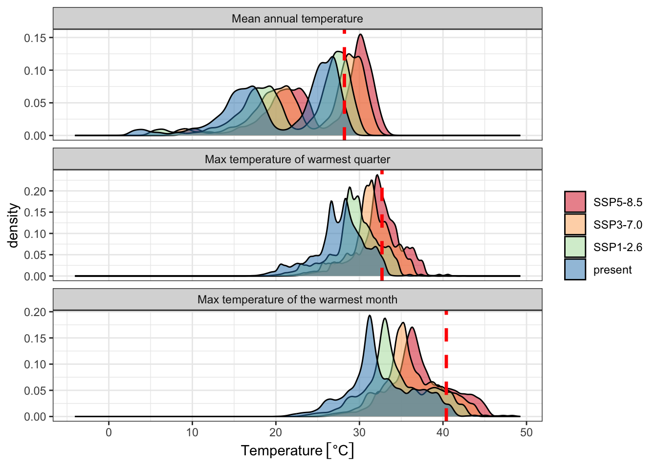
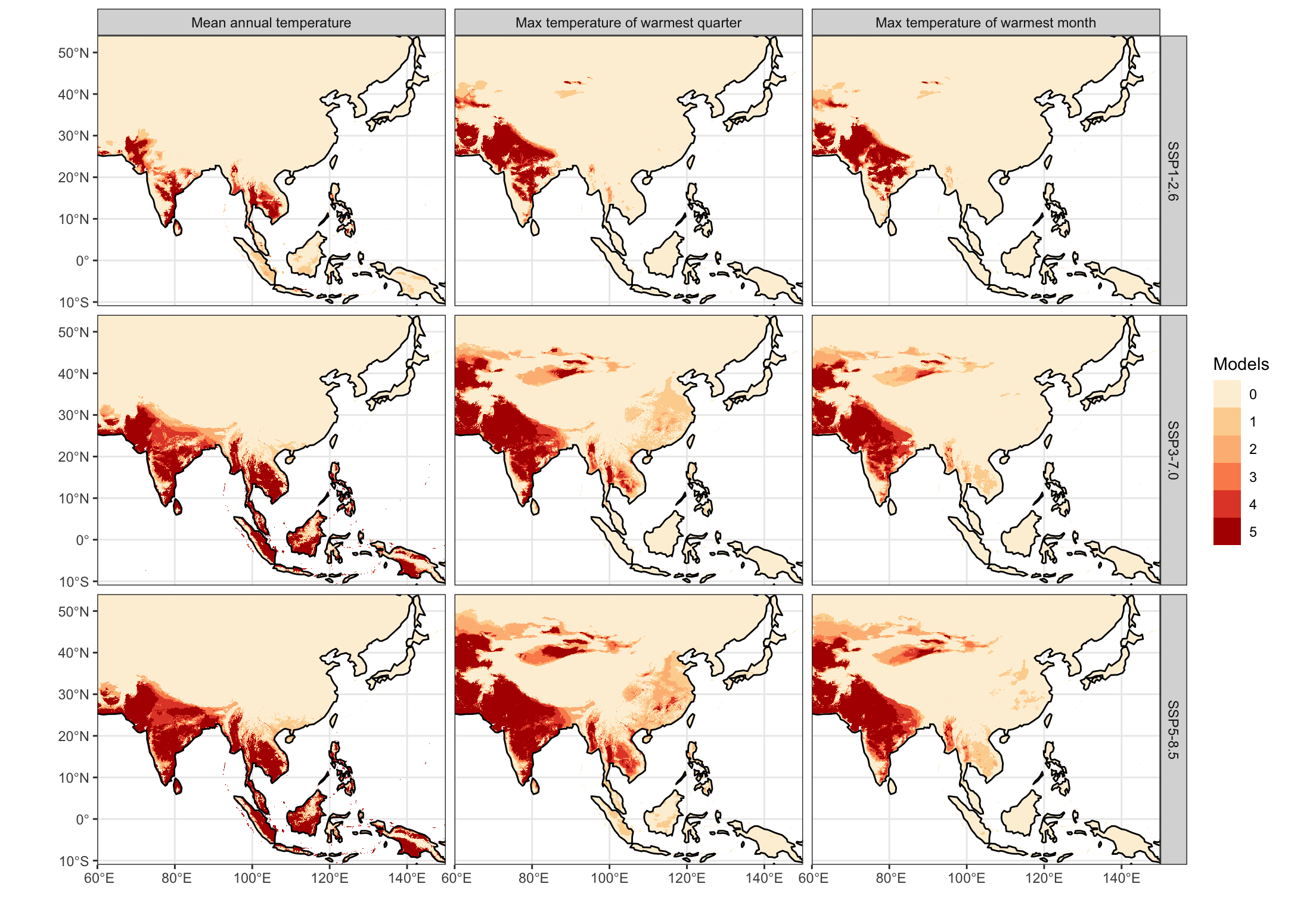
Although rice has spread to warmer environments since its domestication, the magnitude of this change over the past 9,000 years is small relative to anticipated changes by the end of this century. Multiple climate-model projections and future socioeconomic and emissions scenarios show large shifts in annual and warm-season temperatures in regions where rice is currently cultivated intensively, particularly in South, Southeast and Island Southeast Asia (Figure 4). Mean annual temperature will exceed 28℃ for a substantial area of current occurrences in the years 2070-2100. Large parts of South, Southeast, and Island SE Asia will experience temperature conditions for which there is no analogue in the history of the cultivation and domestication of rice over at least the past 9,000 years (Figure 5, Supplementary Figure 11, Supplementary Tables 2-4). Although the extent of these projected shifts vary among climate models and emissions scenarios, the overall direction of this change is consistent (Supplementary Figures 6-8).
In [6]:
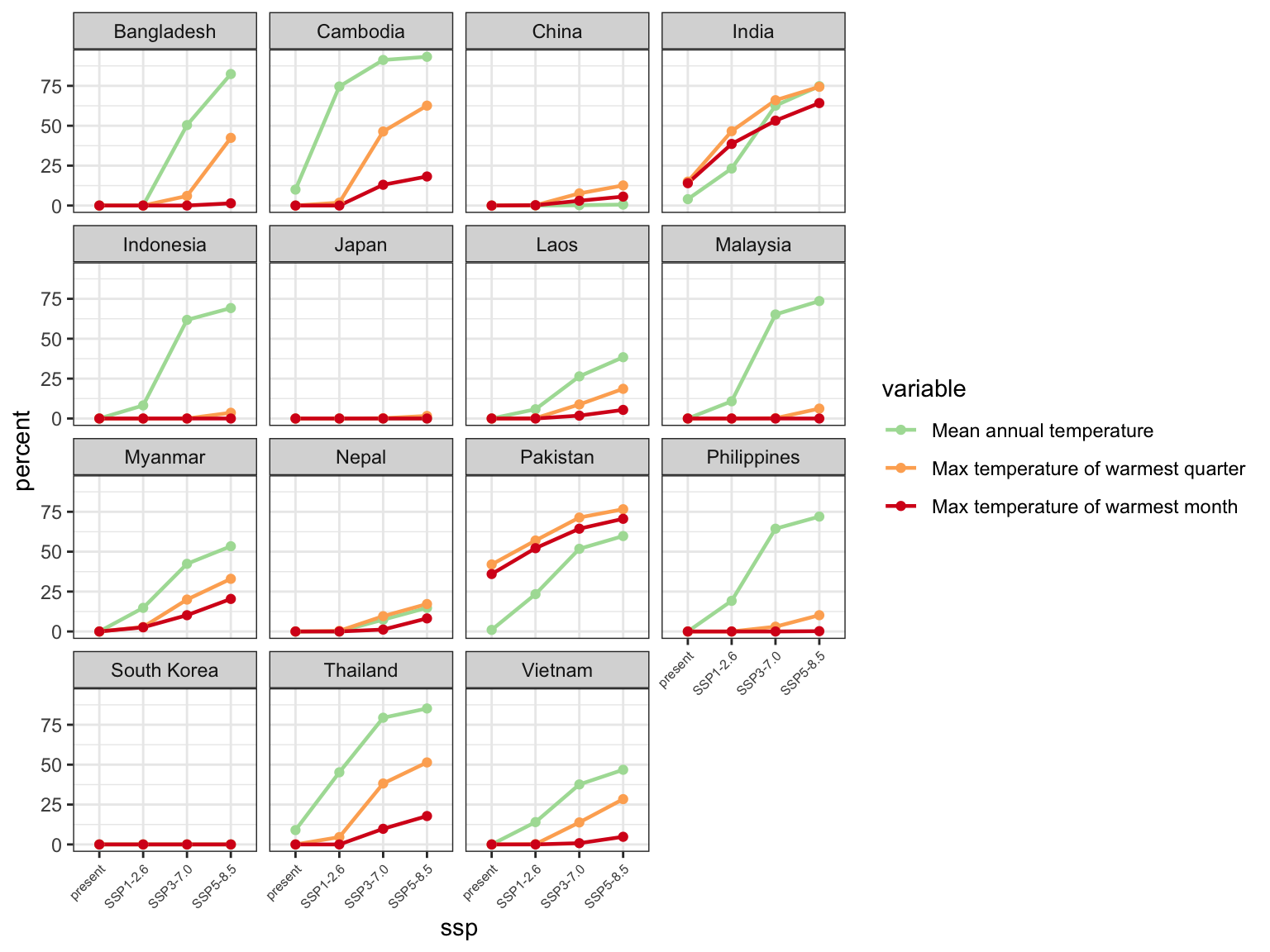
fig5_quantile_data <- quants_mod %>%filter(quantile ==0.975) %>%pivot_longer(-quantile,names_to ='variable',values_to ='temperature') %>%mutate(variable =factor(case_when(variable =='bio1'~'Mean annual temperature', variable =='bio5'~'Max temperature of the warmest month', variable =='bio10'~'Max temperature of warmest quarter'),levels =c('Mean annual temperature', 'Max temperature of the warmest month', 'Max temperature of warmest quarter')))readRDS(here('data/derived/fig_4_data.rds')) %>%bind_rows(pivot_longer(fig2_dat, everything(), names_to ='variable', values_to ='temperature') %>%mutate(ssp ='present')) %>%mutate(ssp =factor(ssp, levels =c('SSP5-8.5', 'SSP3-7.0', 'SSP1-2.6', 'present')),variable =factor(case_when(variable =='bio1'~'Mean annual temperature', variable =='bio10'~'Max temperature of warmest quarter', variable =='bio5'~'Max temperature of the warmest month'),levels =c('Mean annual temperature', 'Max temperature of warmest quarter','Max temperature of the warmest month'))) %>%ggplot(aes(temperature)) +geom_density(aes(fill = ssp), alpha =0.5) +scale_fill_brewer(palette ='Spectral', direction =1, name ='') +facet_wrap(~variable, ncol =1, scales ='free_y') +geom_vline(data = fig5_quantile_data, aes(xintercept = temperature), linetype =2, color ='red', linewidth =1.2) +labs(x ='Temperature')
Figure 4: Predicted changes in biologically relevant temperature indicators over currently cultivated rice areas in Asia, relative to contemporary thermal thresholds (red dashed line). Shared socioeconomic pathways (SSPs) are scenarios of projected socioeconomic global changes used to derive greenhouse gas emission scenarios. SSP1 is a best case scenario where global cooperation and social and technological innovation are able to reduce greenhouse gas emissions. SSP3 is a middle-range scenario characterized by high population growth and global competition that hinders social and technological innovation. SSP5 is a worst-case scenario characterized by rapid economic growth and carbon emissions. All temperature estimates are derived from CMIP6 climate model ensemble mean estimates for the years 2071-2100, selected based on the ISIMIP3b protocol and downscaled by the CHELSA-V2.1 algorithm.
In [7]:
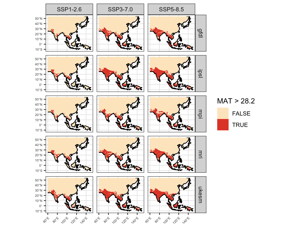
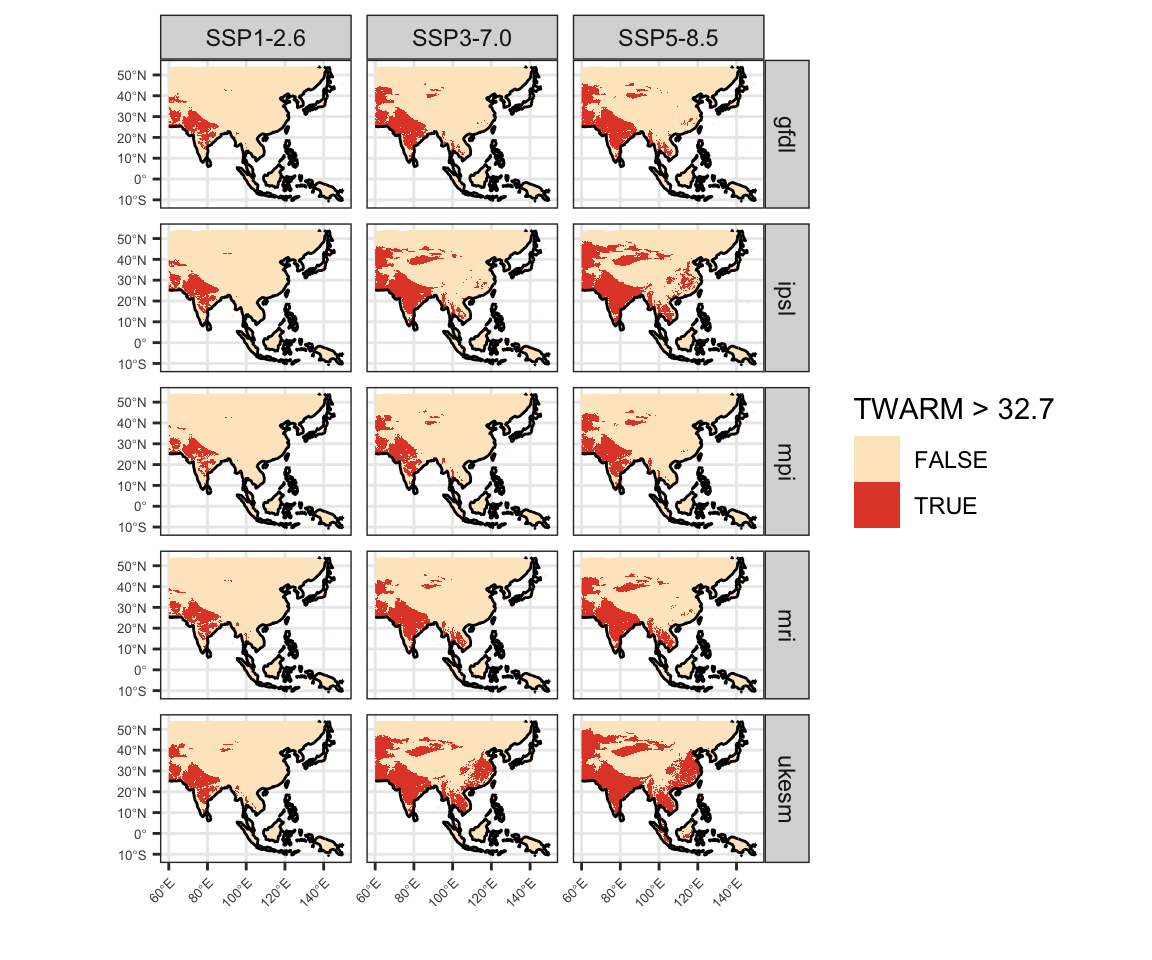
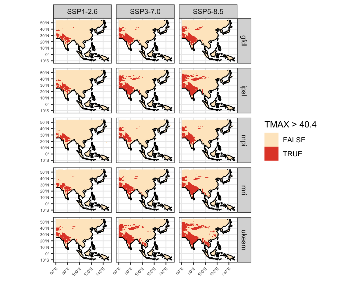
fig5_map_data <- cmip6_maps |>split('variable') %>%mutate(bio1 = bio1 > units::drop_units(bio1_limit),bio10 = bio10 > units::drop_units(bio10_limit),bio5 = bio5 > units::drop_units(bio5_limit) ) %>%rename(`Mean annual temperature`= bio1,`Max temperature of warmest quarter`= bio10,`Max temperature of warmest month`= bio5) %>%merge(name ='variable') |>st_apply(c('x', 'y', 'ssp', 'variable'), sum) %>%mutate(sum =factor(sum)) ggplot() +geom_stars(data = fig5_map_data) +facet_grid(ssp~variable) +scale_fill_brewer(palette ='OrRd', direction =1, name ='Models', na.value =NA, na.translate =FALSE) +geom_sf(data = coasts) +labs(x ='', y ='') +coord_sf(expand =FALSE)
Warning: Removed 3383937 rows containing missing values or values outside the scale
range (`geom_raster()`).
Figure 5: Land areas projected to exceed each temperature threshold by 2071-2100 from CMIP6 simulations, based on the ISIMIP3b protocol and downscaled by CHELSA-V2.1. Color intensity corresponds to the count of climate model ensemble members surpassing the given threshold at each grid cell.
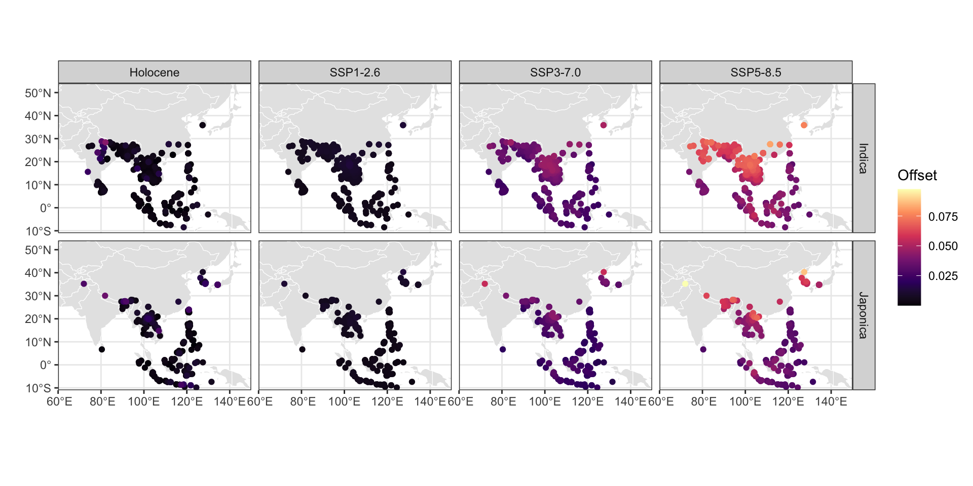
While our spatial analyses reveal clear thermal boundaries in rice distributions, understanding the potential genetic capacity for adaptation provides added context to projected climate shifts. A genetic offset analysis assessing the potential maladaptation of O. sativa subspecies to future climate scenarios, correlating contemporary genetic variation with annual and seasonal temperature, indicates both subspecies are at a significantly higher risk of maladaptation under projected temperature regimes of the coming century (Figure 6). Genetic offset analysis estimates how climatically mismatched rice populations may become under future warming by calculating the multidimensional distance between current allele frequencies and those predicted to be adaptive under projected climate conditions. The analysis produces unitless distance values where larger numbers indicate populations whose current genetic makeup is more divergent from what would be optimal for future climates, suggesting higher vulnerability to climate-driven fitness declines. These distance metrics synthesize information across multiple climate-responsive genetic variants to forecast which populations face the greatest adaptive challenges under temperature increases. When projecting to future climates across Asia, optimal growing locations for rice landraces (traditional crop varieties maintained by farmers and adapted to local conditions) of both subspecies show a greater skew away from the equator in the likeliest emissions scenarios (Supplemental Figure 15). For both japonica and indica, the degree of maladaptation increases with worsening emissions scenarios, but is generally greater than at any point experienced throughout the Holocene.
In [8]:
offset_2.6<-readRDS("data/derived/genetics_plotting/offset_2.6_PC1_K8.rds")offset_7.0<-readRDS("data/derived/genetics_plotting/offset_7.0_PC1_K8.rds")offset_8.5<-readRDS("data/derived/genetics_plotting/offset_8.5_PC1_K8.rds")offset_past <-readRDS("data/derived/genetics_plotting/offset_past_PC1_K8.rds")ind_offset_2.6<-readRDS("data/derived/genetics_plotting/ind_offset_2.6.rds")ind_offset_7.0<-readRDS("data/derived/genetics_plotting/ind_offset_7.0.rds")ind_offset_8.5<-readRDS("data/derived/genetics_plotting/ind_offset_8.5.rds")ind_offset_past <-readRDS("data/derived/genetics_plotting/ind_offset_past.rds")inds_geotagged <-readRDS("data/derived/genetics_plotting/indica_geotagged.rds")japs_geotagged <-readRDS("data/derived/genetics_plotting/japonica_geotagged.rds")# this is the order of the japonica accessions in the genotype matrixjaps <-read.table("data/derived/genetics_plotting/japs_order.txt")inds <-read.table("data/derived/genetics_plotting/inds_order.txt")indica_dat <-tibble(inds$V1, ind_offset_2.6$offset,ind_offset_2.6$distance, ind_offset_7.0$offset,ind_offset_7.0$distance, ind_offset_8.5$offset,ind_offset_8.5$distance, ind_offset_past$offset,ind_offset_past$distance) %>%setNames(c("ID","SSP1-2.6","rona_2.6","SSP3-7.0","rona_7.0","SSP5-8.5","rona_8.5","Holocene", "rona_past" )) %>%left_join(inds_geotagged, by ='ID') %>%select(-starts_with('rona')) %>%pivot_longer(starts_with('SSP') |starts_with('Hol')) %>%arrange(value) %>%rename(scenario = name)japonica_dat <-tibble(japs$V1, offset_2.6$offset,offset_2.6$distance, offset_7.0$offset,offset_7.0$distance, offset_8.5$offset,offset_8.5$distance, offset_past$offset,offset_past$distance) %>%setNames(c("ID","SSP1-2.6","rona_2.6","SSP3-7.0","rona_7.0","SSP5-8.5","rona_8.5","Holocene", "rona_past" )) %>%left_join(japs_geotagged, by ='ID') %>%select(-starts_with('rona')) %>%pivot_longer(starts_with('SSP') |starts_with('Hol')) %>%arrange(value) %>%rename(scenario = name)offset_dat <-list(Indica = indica_dat,Japonica = japonica_dat) %>%bind_rows(.id ='var')ggplot(offset_dat) +geom_sf(data = countries_small, color ='white') +geom_point(aes(LON, LAT, color = value)) +scale_color_viridis_c(option ='magma', name ='Offset') +facet_grid(var~scenario) +labs(x ='', y ='') +coord_sf(expand =FALSE)
Figure 6: Estimated genetic offsets of sampled rice landraces for past and future scenarios relative to current baseline. Each point represents a distinct population sampled for genetic analysis. Higher genetic offsets indicate a greater degree of maladaptation to the particular temperature regime. The “past” scenario reflects the highest modeled temperature at each location over the past 12,000 years. The future scenarios are averaged across all climate models in the ensemble.
Discussion
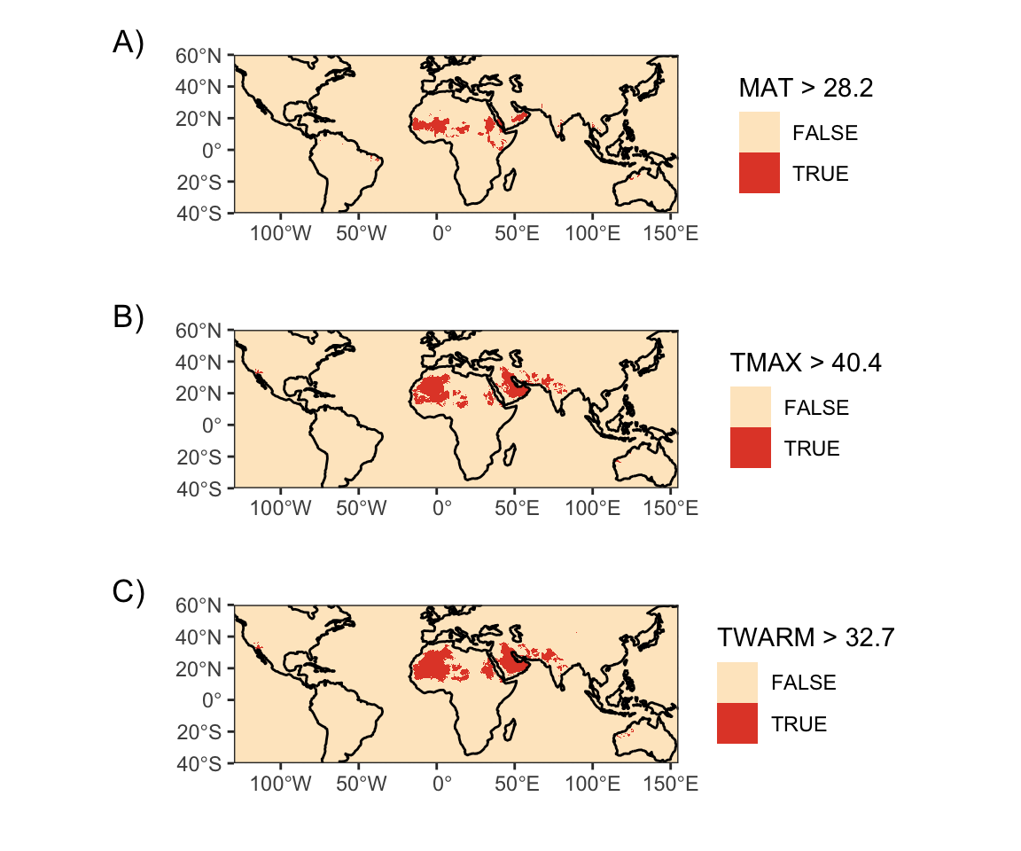
There is a clear upper limit of mean annual temperature over 28℃ and warm-season maximum temperature over 33℃ for rice that has rarely been crossed since its domestication. Forward looking climate projections show that areas that currently house some of the highest densities of rice cultivation on Earth will surpass this limit by the end of this century (Figure 5). Today, 675 million people live in Southeast Asia and 1.9 billion people live in South Asia. By the end of this century, it is estimated that at least this number of people will live in the region that will surpass these thresholds. Today, mean annual temperatures greater than 28℃ are distributed across only a very small area of the planet which includes only a small portion of the gulf desert and the Sahara (54). Beyond the impact of this heat on rice cultivation, this study raises serious concerns about the viability of other temperature-sensitive crops in regions which will be impacted. The predictions for these areas of the world are out of the historic sample of distribution for rice and have no analogue in the present climate.
While some regions, including parts of northern China and southern Russia, may become climatically suitable for rice cultivation and could even see yield gains as temperatures approach current optima (5, e.g. 55, 56), such potential benefits will be highly localized. Even if aggregate yields were to stabilize or increase in some growing regions, they would not offset the immediate livelihood and food security risks faced in regions projected to exceed current thermal limits. Shifting rice production north to regions currently too cold to grow rice will be insufficient to buffer these projected impacts. Beyond the potential for unanticipated social and environmental impacts (57), this response would do little for the billions of people who live in these hotter regions whose lives and livelihoods are directly threatened. This response would also ignore that rice cultivation requires extensive niche construction through the construction of paddies and that abiotic factors such as sufficient water for irrigation and soils which can accommodate paddy rice. Indeed, many areas where rice is currently cultivated are already at the limit of these secondary agronomic adaptations (6). Ethnographic work has shown that in Southeast Asia and China rice paddy soils have been formed over thousands of years of continuous farming which has increased their fertility (58). Such long-term processes of niche construction cannot be easily replaced.
Although we do not directly assess yields, regions projected to warm beyond rice’s historical thermal limits are likely to experience sustained productivity declines without further adaptation, while some cooler areas could benefit as temperatures approach present-day optima. Both outcomes underscore the importance of adaptation strategies to sustain production under shifting climatic conditions. Shifts in planting dates to winter may provide solutions in some regions, but higher temperatures are still a concern as rice is also sensitive to warmer nighttime temperatures in the early growing period (59). While breeding for traits that improve resistance to heat stress, such as early flowering (33), offers some promise, large-scale socio-cultural adaptations to new crop varieties—and, in some cases, shifts in dietary preferences or staple composition (60)—imply significant downstream impacts on regional cultures and economies that can be difficult to anticipate and mitigate ahead of time. Additionally, tropical varieties of O. japonica will likely need to shift northwards to higher latitudes, yet these varieties are highly sensitive to day length, and the development of non-photosensitive temperate O. japonica may have taken thousands of years. More recent efforts, however, such as the Green Revolution in Asia, achieved rapid advances—including the development of non-photosensitive varieties that enabled the expansion of rice cultivation into new latitudes (61). A major breeding objective for the coming decades will thus not only be to develop non-photosensitive varieties of tropical rice but also matching cultivation strategies (e.g. 62) and associated food system strategies and cultural norms.
The stored germplasm of landraces will thus serve as important genetic resources to breed climate-adaptive loci into high-yielding commercial rice varieties (63–65). Compared to modern cultivars, landraces contain higher genetic diversity (66, 67) and adaptations to a wider range of climates (64). This genetic diversity can also be harnessed using traditional varietal mixtures and diversified planting systems (68), where growing complementary crop varieties with different heat tolerances together can buffer against temperature extremes. Maladaptation of rice landraces under future climates may thus be amplified in modern cultivars and cropping systems (69). Although there is uncertainty in genomic offset estimates due to model averaging across climate scenarios and statistical uncertainty in genotype-environment associations, they remain powerful predictors of maladaptation in projected climates (70). A warming climate also threatens wild relatives of rice and the genetic resources they contain, which are currently largely limited to South and Southeast Asia and cannot disperse as quickly without human intervention (1).
Our focus here on annual and seasonal temperature indicators allows for the integration of a broader array of data and provides a more flexible analysis that is less sensitive to uncertainty in cultivar type, growing season, and local management practices. However, future work could explore this variability further by developing new thermal indicators more sensitive to the unique requirements of various cultivars, growing seasons, and agro-ecological contexts. Temperature is not the only climate variable that influences rice growth. Others like soil moisture and solar radiation are also critical to rice growth in ways that, likewise, depend on cultivar type, growing season, and management practices. Extending this analysis to the global and regional climatic drivers of local climate response of these multiple variables, such as the influence of sea surface temperature variability and atmosphere-ocean teleconnections, could provide further opportunities to incorporate long-term climate reconstructions and projections of climate impacts on rice viability. A more precise estimation of the long-range correlations among key climate indicators in space and time, based on long-term insights from the archaeological and paleoclimatological record, would be particularly useful for developing holistic recommendations for future agronomic and genetic adaptations.
Our interdisciplinary approach highlights a pressing reality: the vast historical perspective of rice cultivation combined with past and present climate data provide a sobering outlook for food security during future climatic shifts. Staple food resources entrenched in centuries or millennia of cultural and socio-economic development face unprecedented challenges in the coming decades. The implications of these challenges extend beyond agriculture and resonate through economic systems, trade and migration flows, and deep-rooted cultural practices. The potential displacement of rice cultivation zones suggests not merely a change in global food patterns but a profound disruption of human societies rooted in these agronomic traditions. Before us lies an urgent necessity for international research, collaboration, and adaptive policy-making to strengthen the resilience of this crop that sustains billions.
Materials and Methods
Climate Data
We used high-resolution gridded climate data from version 2.1 of the CHELSA product (71). CHELSA incorporates bias-corrected outputs from the ERA5 reanalysis (72) with high-resolution terrain data using mechanistic relationships between local climate and terrain. Compared to other global gridded climate products, CHELSA offers superior performance in mountainous regions, and its reliance on high-quality reanalysis data instead of raw weather station data ensures greater accuracy and internal consistency among climate variables.
For present-day observed climate, we used the CHELSA V2.1 product spanning the period 1981-2010 at a 1km resolution. We further aggregated the native 1km data to 5km and 10km grids to assess the sensitivity of our results to the scale of the analysis, given the variable spatial support of the contemporary rice extent data. In all cases we used standard temperature indicators used in ecological niche modeling studies (71), derived from monthly climatologies of minimum and maximum temperature, which collectively represent annual means, monthly extremes, and seasonality. Future climate model ensembles were derived from phase six of the Coupled Model Intercomparison Project (CMIP6) (73), using the subset of bias-corrected models and scenarios used in phase 3b of the Inter-Sectoral Impact Model Intercomparison Project (ISIMIP) (74), bilinearly interpolated to the CHELSA V2.1 basemap using the delta change approach (25).
Past climate data were primarily derived from the CHELSA-TraCE21k product, a downscaled version of TraCE-21k simulation of the CCSM3 climate model spanning the last 21,000 years, at 100-year intervals (76). This product uses the older CHELSA V1.2 algorithm, along with a trend-preserving bias correction and topographic correction for shifting ice sheets across the deglacial period. While TraCE-21k has known limitations (77–80), particularly in representing mid-Holocene warmth, it was chosen for its unique combination of high spatial resolution and seasonal temporal resolution necessary for assessing rice cultivation conditions. To validate these findings, we compared our results with other low-resolution mean annual temperature reconstructions that show varying levels of mid-Holocene warmth (81, 82). Despite differences in overall temperature trends, the key patterns in rice cultivation temperature distributions remained consistent between reconstructions (fig. S3).
Contemporary Rice Distribution Data
We collected rice occurrence data from a variety of sources combining information from satellite imagery, administrative statistics, and herbarium collections to assess the sensitivity of our results to various modes of data collection, sampling, spatiotemporal scale, and other potential sources of bias. These three distinct data types sample different aspects of rice distribution with complementary biases. Satellite estimates provide continuous spatial coverage but can misclassify certain land cover types; census data offer detailed regional production information but suffer from administrative reporting issues and boundary effects; herbarium records provide precise, ground-truthed identifications across diverse production systems but show spatial bias in field accessibility and collection priorities. When these data types with different sampling approaches converge on similar thermal limits despite their distinct limitations, this suggests the patterns are less likely to be methodological artifacts. The specific datasets were:
Satellite-based estimates of lowland rice extent in Asia from the International Rice Research Institute (19). This dataset employs high-resolution (500m) presence-absence markers from MODIS observations (2000-2012) and offers relatively uniform sampling across both temperate and tropical regions. It provides a more objective approach than spatially biased occurrence records. However, its coverage is limited to East and Southeast Asia and it may poorly distinguish intercropped wheat and rice in Northeast China and natural wetlands and paddy rice cultivation in Indonesia. To minimize such sampling issues, we aggregated the 500m data into 5km grid cells, dropping occurrences with less than 20% coverage to minimize false positives from low-pixel observations. Subsequent analyses of these data proved robust to the exact resolution and coverage threshold used.
Estimates of paddy rice harvested areas around the year 2000 (20). This dataset, integrates satellite-based estimates of cropland with sub-national statistics for rice harvested areas. It utilizes geospatial cropland maps to downscale harvest area and yield census data and offers global coverage at approximately 10km resolution. Countries that lack detailed administrative data at the subnational level, such as Laos and Kazakhstan, can exhibit overly smoothed areas. The use of harvested area as a metric can be misleading in regions with multiple annual harvests, leading to double or triple counting, but this is mitigated when converted to binary occurrence data.
Geolocated, point-based occurrence records for rice and its wild progenitor synthesized from previous studies (2, 18, 21, 22), originally sourced from GBIF, the Rice Haplotype Map project, and other datasets based on herbarium specimens or germplasm samples from international genebank databases. Given their direct identification, these occurrence records generally offer greater reliability than area-averaged crop occurrences derived from satellites and sub-national statistics. Nonetheless, they are susceptible to spatial sampling bias. For instance, regions like China are underrepresented in GBIF in terms of sampling effort compared to neighboring countries with similar geographical extent, and herbarium collections may more accurately sample upland rice varieties at the expense of larger paddy fields. After creating the full combined datasets, geolocations were checked for anomalous entries then thinned to a uniform grid to minimize irregular spatial sampling.
We extracted the contemporary CHELSA climate data at each set of occurrence points for each data type to calculate temperature distributions and quantiles. We explored various combinations of grid/point resolution for the climate and occurrence datasets from 1-10km, but found this did not impact the upper temperature threshold estimates.
Archaeological Rice Distribution Data
We used past rice occurrence data sourced from archaeological sites in Asia, as synthesized in (83) and (13) and primarily derived from version 2 (15) and 3 (Dorian Fuller 2023, personal communication) of the Rice Archaeological Database. We also included observations from (14) to increase data coverage in Japan. These records are typically of botanical remains, believed to represent O. sativa japonica from these archaeological sites, with less intensive sampling of indica varieties from northern India. However, based on their chronology, some occurrences might instead reflect cultivation of wild-type O. rufipogon or O. nivara. After data harmonization—which involved eliminating potential outliers, correcting misclassifications, and removing duplicated site data (see supplemental analysis code repository for the reproducible workflow)—we were left with 1,595 dates from 803 archaeological sites. These datasets comprise a mixture of direct radiocarbon dates on rice remains, alongside dates for archaeological phases associated with rice remains that were not directly dated. For these indirectly dated samples, we used median dates and minimum/maximum date ranges for the archaeological strata or contexts in which the rice remains were found. We employed the Intcal20 calibration curve for recalibrating all radiocarbon dates, barring a single site in the southern hemisphere where we utilized SHcal20. We then extracted temperature variables from the CHELSA-TraCE21k v1.0 dataset at each sampled location in time and space. To account for chronological uncertainty, we generated 5,000 bootstrap replicates, sampling from the radiocarbon dates’ posterior density distribution and a uniform density for the dates based on archaeological phases. Finally, we constructed unique kernel density estimates of the temperature distributions at each rice occurrence point for every bootstrap replicate and temperature variable.
Genetic Offset Analysis
To assess the adaptive capacity of rice varieties beyond simple distributional limits, we performed a genetic offset analysis to evaluate the potential maladaptation of Oryza sativa subspecies indica and japonica under projected climate change scenarios. Genetic offset metrics provide a complementary perspective to geographical threshold analyses by identifying where genetic adaptation may or may not keep pace with changing thermal conditions. Landraces are representative of the extant genetic diversity of crop species, and frequently exhibit local adaptations from sustained cultivation in specific geographic localities. We leveraged previously published genomic datasets of geotagged rice landraces belonging to the subspecies O. sativa ssp. Indica(18) and O. sativa ssp. Japonica(84), containing genome-wide biallelic single nucleotide polymorphisms (SNPs) filtered for quality and imputed for missing genotypes. The workflow entailed a gene-environment association analysis focusing on the first principal component of the three temperature variables (MAT, TWARM, TMAX), which explained over 84% of the environmental variance across the locations of both rice subspecies. Using the first principal component addresses multicollinearity among the temperature variables while retaining most environmental variation. The gene-environment association analysis was performed using the lfmm2 function from the R package LEA (v3.12.2)—on the two subspecies separately—to identify variants associated with variation in temperature (85). To correct for population structure in the GEA, we provided the number of ancestral populations, K, as the number of latent factors in our latent factor mixed models (85). We selected the number of ancestral populations based on the number of principal components of the genotype matrix that explain a large proportion of the variance, the cross-entropy—a measure of model fit—of different values of K, and information from prior studies (18, 84). Variants identified in the GEA were clumped within 100 kilobases of each other, selecting the variant with the lowest p-value as the candidate SNP from each linkage group. The genetic offset, indicative of maladaptation to predicted climates (70), was calculated using these loci. These offset values indicate the Euclidean distance between current genomic composition and the composition theoretically required for adaptation to projected climate conditions. We averaged model predictions across multiple climate models (UKESM, MRI, IPSL, etc.) in the ensemble for each Shared Socioeconomic Pathway (SSP).
We used the genetic.offset function of the R package LEA (85) to calculate genomic offset statistics for rice landraces of O. sativa ssp. Indica and O. sativa ssp. Japonica while considering the temperature-associated variants as putative adaptive variants under the SSP1, SSP3, and SSP5 projected pathways that are used to derive greenhouse gas emission scenarios. We also calculated genomic offset statistics under the maximum estimated temperature at each location in the past 12,000 years.
To make predictions about where the climate is likely to be optimal for rice-growing in the future, we sampled 10,000 grids from across Asia and calculated genomic offset scores for each individual in the environment of each grid, for the three SSP scenarios. We interpret the grid with the lowest offset score as a possible future optimal location for each rice individual. As a measure of the extent of movement that would be required for adaptation, we subtract the absolute value of the current latitude of each rice individual from the absolute value of the centroid latitude of the optimal grid; positive values of this absolute latitudinal distance indicate movement away from the equator.
L. L. Sloat, S. J. Davis, J. S. Gerber, F. C. Moore, D. K. Ray, P. C. West, N. D. Mueller, Climate adaptation by crop migration. Nature Communications11, 1243 (2020).
Y. Gao, J. Cui, X. Zhang, G. Hoogenboom, D. Wallach, Y. Huang, S. Reis, T. Lin, B. Gu, Cost-effective adaptations increase rice production while reducing pollution under climate change. Nature Food6, 260–272 (2025).
V. Masson-Delmotte, P. Zhai, A. Pirani, S. L. Connors, C. Péan, S. Berger, N. Caud, Y. Chen, L. Goldfarb, M. Gomis, others, Climate change 2021: The physical science basis. Contribution of working group I to the sixth assessment report of the intergovernmental panel on climate change2 (2021).
R. M. Gutaker, S. C. Groen, E. S. Bellis, J. Y. Choi, I. S. Pires, R. K. Bocinsky, E. R. Slayton, O. Wilkins, C. C. Castillo, S. Negrão, M. M. Oliveira, D. Q. Fuller, J. A. d’Alpoim. Guedes, J. R. Lasky, M. D. Purugganan, Genomic history and ecology of the geographic spread of rice. Nature Plants6, 492–502 (2020).
19.
A. Nelson, M. K. Gumma, A map of lowland rice extent in the major rice growing countries of Asia (2015).
J. Ramirez-Villegas, C. K. Khoury, H. A. Achicanoy, M. V. Diaz, A. C. Mendez, C. C. Sosa, Z. Kehel, L. Guarino, M. Abberton, J. Aunario, B. A. Awar, J. C. Alarcon, A. Amri, N. L. Anglin, V. Azevedo, K. Aziz, G. L. Capilit, O. Chavez, D. Chebotarov, D. E. Costich, D. G. Debouck, D. Ellis, H. Falalou, A. Fiu, M. E. Ghanem, P. Giovannini, A. J. Goungoulou, B. Gueye, A. I. E. Hobyb, R. Jamnadass, C. S. Jones, B. Kpeki, J.-S. Lee, K. L. McNally, A. Muchugi, M.-N. Ndjiondjop, O. Oyatomi, T. S. Payne, S. Ramachandran, G. Rossel, N. Roux, M. Ruas, C. Sansaloni, J. Sardos, T. D. Setiyono, M. Tchamba, I. van den Houwe, J. A. Velazquez, R. Venuprasad, P. Wenzl, M. Yazbek, C. Zavala, State of ex situ conservation of landrace groups of 25 major crops. Nature Plants8, 491–499 (2022).
D. N. Karger, O. Conrad, J. Böhner, T. Kawohl, H. Kreft, R. W. Soria-Auza, N. E. Zimmermann, H. P. Linder, M. Kessler, Data from: Climatologies at high resolution for the earth’s land surface areas. doi: 10.5061/dryad.kd1d4 (2018).
25.
P. Brun, N. E. Zimmermann, C. Hari, L. Pellissier, D. N. Karger, “Global climate-related predictors at kilometre resolution for the past and future” (2022); https://doi.org/10.5194/essd-2022-212.
S. M. Gourdji, K. L. Mathews, M. Reynolds, D. B. Lobell, S. M. Gourdji, An assessment of wheat yield sensitivity and breeding gains in hot environments. (2012).
X. Huang, N. Kurata, X. Wei, Z.-X. Wang, A. Wang, Q. Zhao, Y. Zhao, K. Liu, H. Lu, W. Li, Y. Guo, Y. Lu, C. Zhou, D. Fan, Q. Weng, C. Zhu, T. Huang, L. Zhang, Y. Wang, L. Feng, H. Furuumi, T. Kubo, T. Miyabayashi, X. Yuan, Q. Xu, G. Dong, Q. Zhan, C. Li, A. Fujiyama, A. Toyoda, T. Lu, Q. Feng, Q. Qian, J. Li, B. Han, A map of rice genome variation reveals the origin of cultivated rice. Nature490, 497–501 (2012).
C. Xu, T. A. Kohler, T. M. Lenton, J.-C. Svenning, M. Scheffer, Future of the human climate niche. Proceedings of the National Academy of Sciences, 1–6 (2020).
55.
X. Wang, C. Zhao, C. Müller, C. Wang, P. Ciais, I. Janssens, J. Peñuelas, S. Asseng, T. Li, J. Elliott, others, Emergent constraint on crop yield response to warmer temperature from field experiments. Nature Sustainability3, 908–916 (2020).
56.
S. Minoli, J. Jägermeyr, S. Asseng, A. Urfels, C. Müller, Global crop yields can be lifted by timely adaptation of growing periods to climate change. Nature Communications13, 7079 (2022).
W. Willett, J. Rockström, B. Loken, M. Springmann, T. Lang, S. Vermeulen, T. Garnett, D. Tilman, F. DeClerck, A. Wood, others, Food in the anthropocene: The EAT–lancet commission on healthy diets from sustainable food systems. The lancet393, 447–492 (2019).
61.
A. R. L. Eliazer Nelson, K. Ravichandran, U. Antony, others, The impact of the green revolution on indigenous crops of india. Journal of Ethnic Foods6, 1–10 (2019).
P. Brun, N. E. Zimmermann, C. Hari, L. Pellissier, D. N. Karger, CHELSA-BIOCLIM+ a novel set of global climate-related predictors at kilometre-resolution. https://doi.org/10.16904/envidat.332.
72.
H. Hersbach, B. Bell, P. Berrisford, S. Hirahara, A. Horányi, J. Muñoz-Sabater, J. Nicolas, C. Peubey, R. Radu, D. Schepers, A. Simmons, C. Soci, S. Abdalla, X. Abellan, G. Balsamo, P. Bechtold, G. Biavati, J. Bidlot, M. Bonavita, G. De Chiara, P. Dahlgren, D. Dee, M. Diamantakis, R. Dragani, J. Flemming, R. Forbes, M. Fuentes, A. Geer, L. Haimberger, S. Healy, R. J. Hogan, E. Hólm, M. Janisková, S. Keeley, P. Laloyaux, P. Lopez, C. Lupu, G. Radnoti, P. de Rosnay, I. Rozum, F. Vamborg, S. Villaume, J.-N. Thépaut, The ERA5 global reanalysis. Quarterly Journal of the Royal Meteorological Society146, 1999–2049 (2020).
Z. Liu, J. Zhu, Y. Rosenthal, X. Zhang, B. L. Otto-Bliesner, A. Timmermann, R. S. Smith, G. Lohmann, W. Zheng, O. Elison Timm, The holocene temperature conundrum. Proceedings of the National Academy of Sciences, 1–5 (2014).
Competing interests: The authors declare that they have no competing interests.
Data and materials availability: All analyses carried out in R(86). The analysis is run via reproducible .qmd notebooks available here. All data required to reproduce the main analysis and figures are included with the linked code repository or available from public sources referenced therein.
Supplementary Materials
Supplementary Materials for Projected warming will exceed the long-term thermal limits of rice cultivation
Nicolas Gauthier, Ornob Alam, Michael D. Purugganan, Jade d’Alpoim Guedes
Figure 7: Present day geographic distribution of temperature thresholds in CHELSA V2.1 data. A) Mean annual temperature greater than 28.2°C. B) Mean maximum temperature of the warmest month greater than 40.4°C. C) Mean maximum temperature of the warmest quarter greater than 32.7°C.
`stat_bin()` using `bins = 30`. Pick better value with `binwidth`.
Figure 8: A) Bootstrapped kernel density estimates of rice’s thermal extent throughout the Holocene. Bootstrap resampling accounts for uncertainty in radiocarbon and phase-based dating of archaeological rice finds. Contemporary temperature thresholds indicated in red. B) Estimated 97.5% quantiles from the bootstrapped dataset. Contemporary quantiles indicated in red.
In [11]:
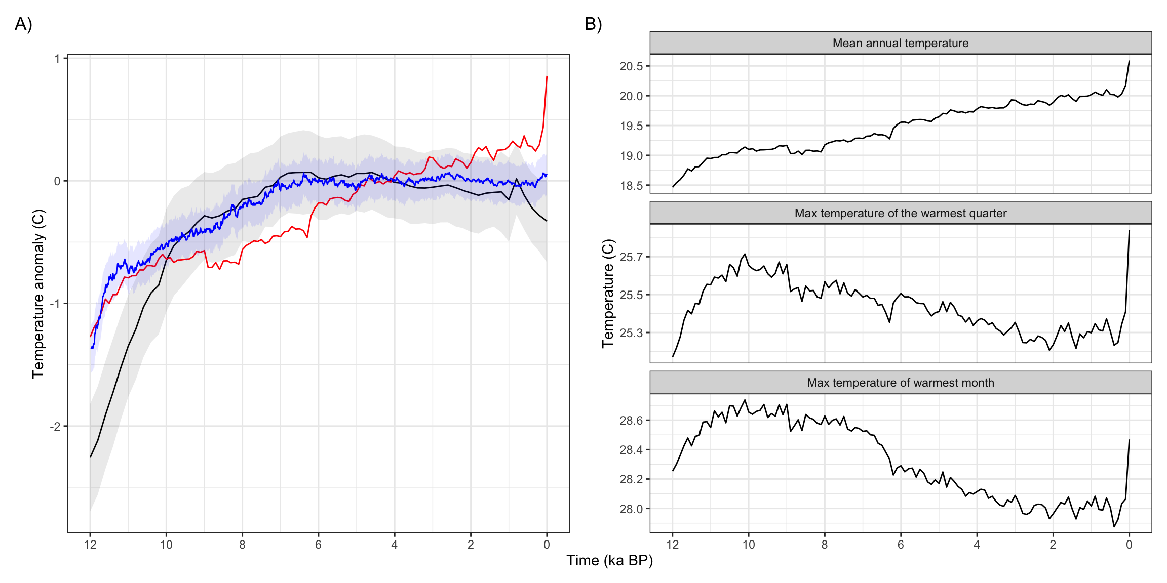
trace_ts <-read_rds(here('data/derived/trace_ts.rds'))a <- trace_ts |>pivot_longer(-time) |>mutate(name =factor(case_when(name =='bio1'~'Mean annual temperature', name =='bio5'~'Max temperature of warmest month', name =='bio10'~'Max temperature of the warmest quarter'),levels =c('Mean annual temperature', 'Max temperature of the warmest quarter','Max temperature of warmest month'))) |>ggplot() +geom_line(aes(time, value, group = name)) +facet_wrap(~name, scales ='free_y', ncol =1) +labs(x ='Time (ka BP)', y ='Temperature (C)') +scale_x_reverse(breaks =seq(0, 12, 2)) +theme_bw()# Calculate the area-weighted averaged temperatures and uncertainties from the Erb et al. reconstruction and save the results.erb_rast <-read_rds(here('data/derived/erb_rast.rds'))erb_area_total <-st_area(erb_rast) |>pull(area) |>sum()erb_ts <- (erb_rast *st_area(erb_rast)) |>st_apply(3, sum) |>as_tibble() |>mutate(across(-ages, ~units::drop_units(.x / erb_area_total)),time = ages /1000) |>select(-ages)# Do the same for the LGMR, although this is more complicated as we have to calculate the anomalies by hand for comparison to Erb.lgmr_rast <-read_rds('data/derived/lgmr_rast.rds')lgmr_mean_reference <- lgmr_rast |>filter(between(time, 3000, 5000)) |>st_apply(1:2, mean)lgmr_sd_reference <- lgmr_rast |>filter(between(time, 3000, 5000)) |>select(sat_std) |># we need to account for uncertainty in the reference period toost_apply(1:2, function(x) sqrt(sum(x^2) /11) /sqrt(11)) # 11 is the number of time stepslgmr_uncertainty <-sqrt(lgmr_rast['sat_std'] ^2+ lgmr_sd_reference ^2)lgmr_rast_anom <- lgmr_rast['sat'] - lgmr_mean_reference['sat']lgmr_anomalies <-c(anom = lgmr_rast_anom,anom_upper = lgmr_rast_anom + lgmr_uncertainty,anom_lower = lgmr_rast_anom - lgmr_uncertainty)lgmr_area_total <-st_area(lgmr_rast_anom) |>as_tibble() |>pull(area) |>sum()lgmr_anom_ts <- (lgmr_anomalies *st_area(lgmr_rast_anom)) |>st_apply(3, sum) |>as_tibble() |>mutate(across(-time, ~units::drop_units(.x / lgmr_area_total)),time = time /1000)b <-ggplot(data = lgmr_anom_ts, aes(x = time)) +geom_line(aes(y = anom)) +geom_ribbon(aes(ymin = anom_lower, ymax = anom_upper), alpha =0.1) +geom_line(data = trace_ts, aes(x = time, y = bio1 -19.737), color ='red') +geom_line(data = erb_ts, aes(y = sat_mean), color ='blue') +geom_ribbon(data = erb_ts, aes(ymin = sat_low , ymax = sat_high), alpha =0.1, fill ='blue') +scale_x_reverse(breaks =seq(0, 12, 2)) +labs(x ='Time (ka BP)', y ='Temperature anomaly (C)') b + a +plot_layout(guides ='collect', axes ='collect') +plot_annotation(tag_levels ='A', tag_suffix =')')
Figure 9: Comparison of Holocene temperature trends over Asia from transient climate models and reconstructions. A) Holocene trends in mean annual temperature, relative to the 3-5ka mean, from Osman et al. 2021 (black, one standard deviation uncertainty in grey), Erb et al. 2022 (blue), and CHELSA-TraCE21k (red). B) Comparison of annual, seasonal, and monthly temperature trends over Asia from CHELSA-TraCE21k.
New names:
• `time` -> `time...9`
• `time` -> `time...14`
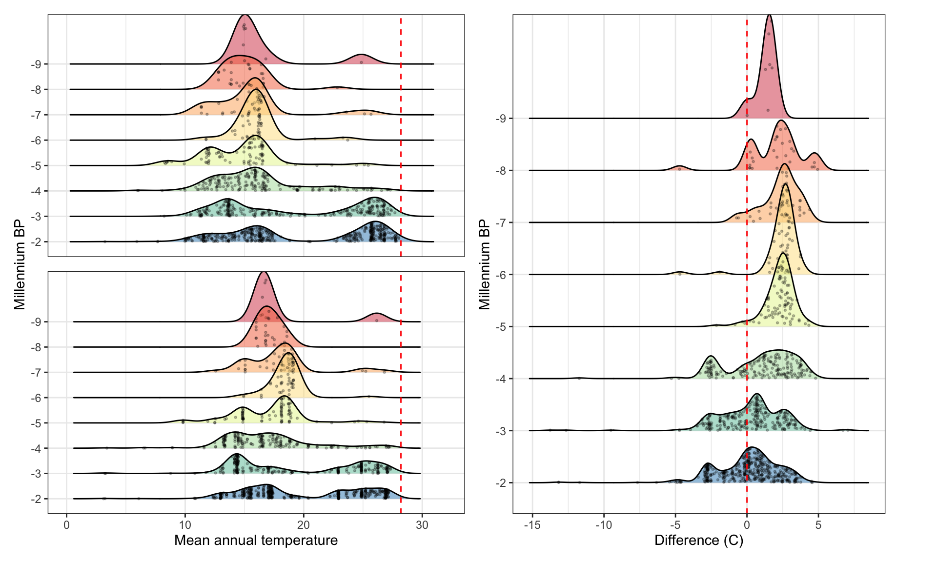
arch_dens_mat <- arch_trace_dat %>%ggplot(aes(MAT, mil)) +scale_y_discrete(limits = rev) +geom_density_ridges(aes(fill = mil), panel_scaling =TRUE, scale =2, alpha =0.5, jittered_points =TRUE, point_alpha =0.25, point_size =0.5) +labs(y ='Millennium BP', x ='Mean annual temperature') +geom_vline(xintercept =as.numeric(bio1_limit), linetype =2, color ='red') +scale_fill_brewer(palette ='Spectral', guide ='none') +scale_x_continuous(limits =c(0, 32))arch_dens_lgmr <- lgmr_extract_test %>%ggplot(aes(sat, mil)) +scale_y_discrete(limits = rev) +geom_density_ridges(aes(fill = mil), panel_scaling =TRUE, scale =2, alpha =0.5, jittered_points =TRUE, point_alpha =0.25, point_size =0.5) +labs(y ='Millennium BP', x ='Mean annual temperature') +geom_vline(xintercept =as.numeric(bio1_limit), linetype =2, color ='red') +scale_fill_brewer(palette ='Spectral', guide ='none') +scale_x_continuous(limits =c(0, 32))# the difference between Chelsa-TraCE and LGMR ensemble mean at each point in time/spacearch_dens_diff <- lgmr_extract_test %>%ggplot(aes(sat - MAT, mil)) +scale_y_discrete(limits = rev) +geom_density_ridges(aes(fill = mil), panel_scaling =TRUE, scale =2, alpha =0.5, jittered_points =TRUE, point_alpha =0.25, point_size =0.5) +labs(y ='Millennium BP', x ='Difference (C)') +geom_vline(xintercept =0, linetype =2, color ='red') +scale_fill_brewer(palette ='Spectral', guide ='none')# why don't the tags work here?(arch_dens_mat / arch_dens_lgmr +plot_layout(axes ='collect')) | arch_dens_diff +plot_layout(widths =c(1, .1)) +plot_annotation(tag_levels ='A', tag_suffix =')')
Picking joint bandwidth of 0.976
Picking joint bandwidth of 0.833
Warning: Removed 3 rows containing non-finite outside the scale range
(`stat_density_ridges()`).
Picking joint bandwidth of 0.481
Figure 10: Kernel density estimates of the thermal distribution by millennium across two different temperature datasets, with raw data points indicated in black and contemporary rice thermal limits in red. A) Temperature data are derived from CHELSA-TraCE21k V1.0 (Karger et al. 2023) (same as Figure 3b in main text). B) Temperature data derived from the Last Glacial Maximum Reanalysis (LGMR) dataset (Osman et al. 2022). C) Difference in kernel density estimates of mean annual temperature (MAT) between the CHELSA-TraCE21k and LGMR datasets.
Warning: Removed 5639895 rows containing missing values or values outside the scale
range (`geom_raster()`).
Figure 13: Predicted changes in mean maximum temperature of the warmest quarter over currently cultivated rice areas in Asia for multiple CMIP6 ensemble members.
Warning: Removed 5639895 rows containing missing values or values outside the scale
range (`geom_raster()`).
Figure 14: Predicted changes in mean maximum temperature of the warmest month over currently cultivated rice areas in Asia for multiple CMIP6 ensemble members.
In [17]:
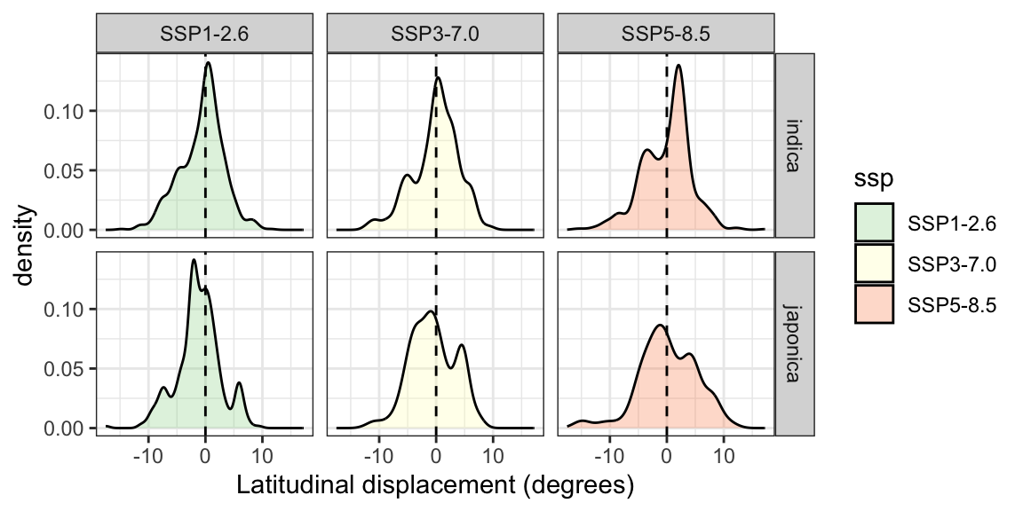
list(japonica =readRDS(here('data/derived/japonica_lat_shift.rds')),indica =readRDS(here('data/derived/indica_lat_shift.rds'))) |>bind_rows(.id ='landrace') |>mutate(ssp =case_when(name =='diff2.6'~'SSP1-2.6', name =='diff7.0'~'SSP3-7.0', name =='diff8.5'~'SSP5-8.5')) |>ggplot(aes(x = value, fill = ssp)) +geom_density(alpha =0.3) +facet_grid(landrace ~ ssp) +geom_vline(xintercept =0, linetype =2) +scale_fill_brewer(palette ='Spectral', direction =-1) +labs(x ='Latitudinal displacement (degrees)')
Figure 15: Estimated displacement of the optimal growing location of rice landraces away from the equator, based on genetic offset analysis across three future temperature scenarios. The x-axis indicates the difference between the absolute projected latitude in the future scenario and the absolute latitude today, with positive values indicating a shift in the optimal growing location of a given population away from the equator.
Table 1: Present-day rice extent quantiles (in °C) across three datasets of varying resolution and spatiotemporal support, compared to those calculated from archaeological sites in Asia throughout the Holocene.